
Measurement Results
INA gain
There are two ways to verify our INA gain. One is giving a sine wave input for the INA and seeing how large we get at the output and getting the ratio of the output peak divided by the input peak. Based on observation on the oscilloscope we can find out that the gain is about 83-81, which is around 38.83dB. Another way is like what we did in Cadence AC simulation, plot out the frequency response and see how it matches with the sine-wave input performance. At the end, both measurement methods show quite the same result for the INA gain.
For direct sine-wave input simulation, what we need to do is set up a fully differential input with its difference as a sine-wave signal. This can be realized through two synchronous waveform generators. For the output signal, we can directly read it on the oscilloscope measure its pk-pk value, and divide it by the initial difference input we set.
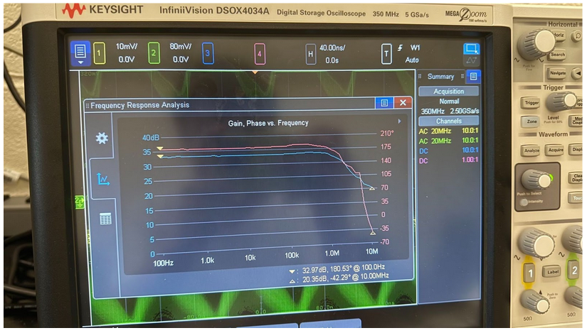
Fig 1. INA Gain Results
For the INA gain, we measure it with the help of a waveform generator from an oscilloscope. We utilize the frequency response analysis (FRA) function on it and use its own waveform generator to provide excitation for INA. We give a small input amplitude which is around 20mV (minimum value of waveform generator), and since our INA is a fully differential structure, but the FRA can only work for the single-ended circuit, we need to manually add 6dB gain onto our gain result since the output is just measured on one side.
What we can see from this plot is that the gain response is 32.97dB for DC and low frequency. After adding 6dB, it is quite close to what we get from the sine-wave input method, which is 38.97dB for the INA gain.
With these 2 methods, we can prove that our INA gain design is quite robust and can give us a stable 38.9dB low-frequency gain.
CMRR
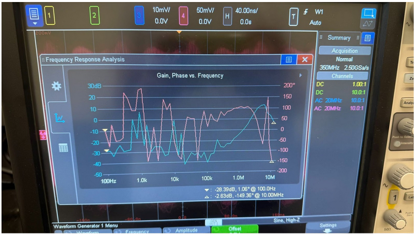
Fig 2. CMRR Results
For the CMRR definition, we know that it should be the ratio of differential gain (Add) divided by the common mode to differential (Acd) gain. We already get our differential gain as 38.9dB as above and for Acd, the way we measure it is by giving a common signal with one common-mode DC to the differential input and measuring its output difference. Since the signal we care about is really small, which means if we try to directly use same sine-wave input injected into the two ports of our INA, we won't see anything on the oscilloscope since the oscilloscope noise would even be larger than what we have for output from common-mode input. We finally try to use the FRA method to see its ac response again on the oscilloscope, and what is shown on the graph is like -28.39dB at the frequency range we care about, which means our real CMRR in this case would be close to 65dB. However, we should notice that the oscilloscope accuracy may not be that good so it is really hard to see the Acd through an oscilloscope. We might need an attenuator for input attenuation since input of 20mV (which is the smallest one from the waveform generator of an oscilloscope may make our amplifier get saturated in this case).
ADC
ENOB
We used Digilent to input ADC differential sine waves and capture the digital outputs. Spectrum is computed in Matlab using a Discrete Fourier Transform. The result is shown below although it indicates that spectrum leakage happens. We need to apply window functions to optimize. With spectrum leakage, the ENOB is 7.52 bits. In addition, the signal generator of the Digilent also is noisy. We can implement a filter before sending the input signal to the ADC to optimize the testing result.
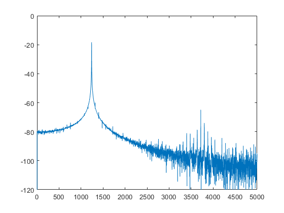
Fig 3. DFT Spectrum
INL & DNL
We use a very slow sine wave input (600mV peak to peak) and collect the result. The result shows that we have two missing codes. DNL is ±1 LSB and INL is ±2 LSB.
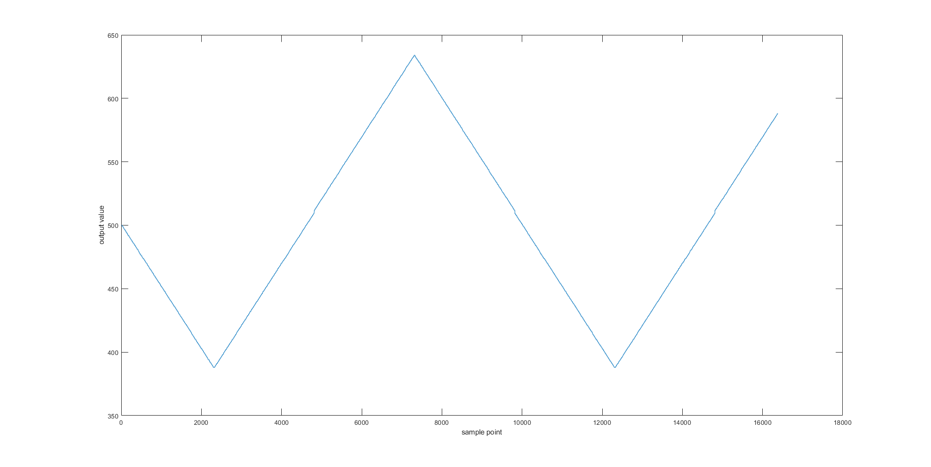
Fig 4. DFT Spectrum
Whole System Testing Setup
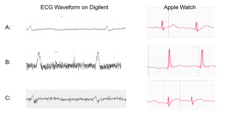
Fig 3. Results comparison
The middle wave of the ECG signal is what we usually call 'R wave', it should be the highest peak and if you do a measurement for the time interval within 2 peaks you can easily get a good estimation of your heart wave. There should be 2 small droops on the left and right side of the middle, which we usually call 'Q wave' and 'S wave', respectively. While for the bump next to the right droop, is usually called 'T wave'. Different waves with different shapes can give us different information to know how our heart is functioning. By future DSP on these data, either you or professional doctors can have a good estimation on your heart health.
In this experiment, we compared the ECG waveform we get from the digilent bus and the ECG waveform we get directly on the Apple Watch S8.
Basically, the shapes are quite the same. For different people, like B, he has an extremely high peak for R wave, which gets matched in both digilent bus and Apple watch. As for C, it is also obvious that it has a relatively obvious droop after the middle peak. This is also the same in both Apple Watch and digilent output.
To control the variables, we use the same gain of PGA on these 3 testers. Some people may have a strong ECG signal or maybe a good connection to the electrode to get a relatively larger peak shown on the waveform.