
Simulation Results
ADC simulation results:
Figure. 1 show the testbench of the whole ADC test, with ideal clock frequency input and we can have any input signal frequency. Therefore, we can have perfect coprime sampling results.
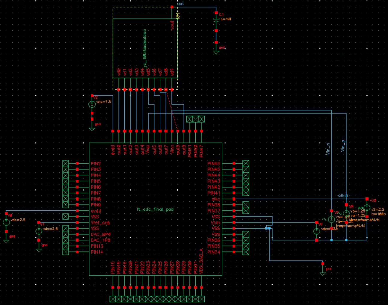
Figure. 1 ADC Testbench
The Figure. 2 is the result of the testbench calculating ENOB with coprime frequency. The ENOB is 9.88bits and several tones can been seen in the figure.
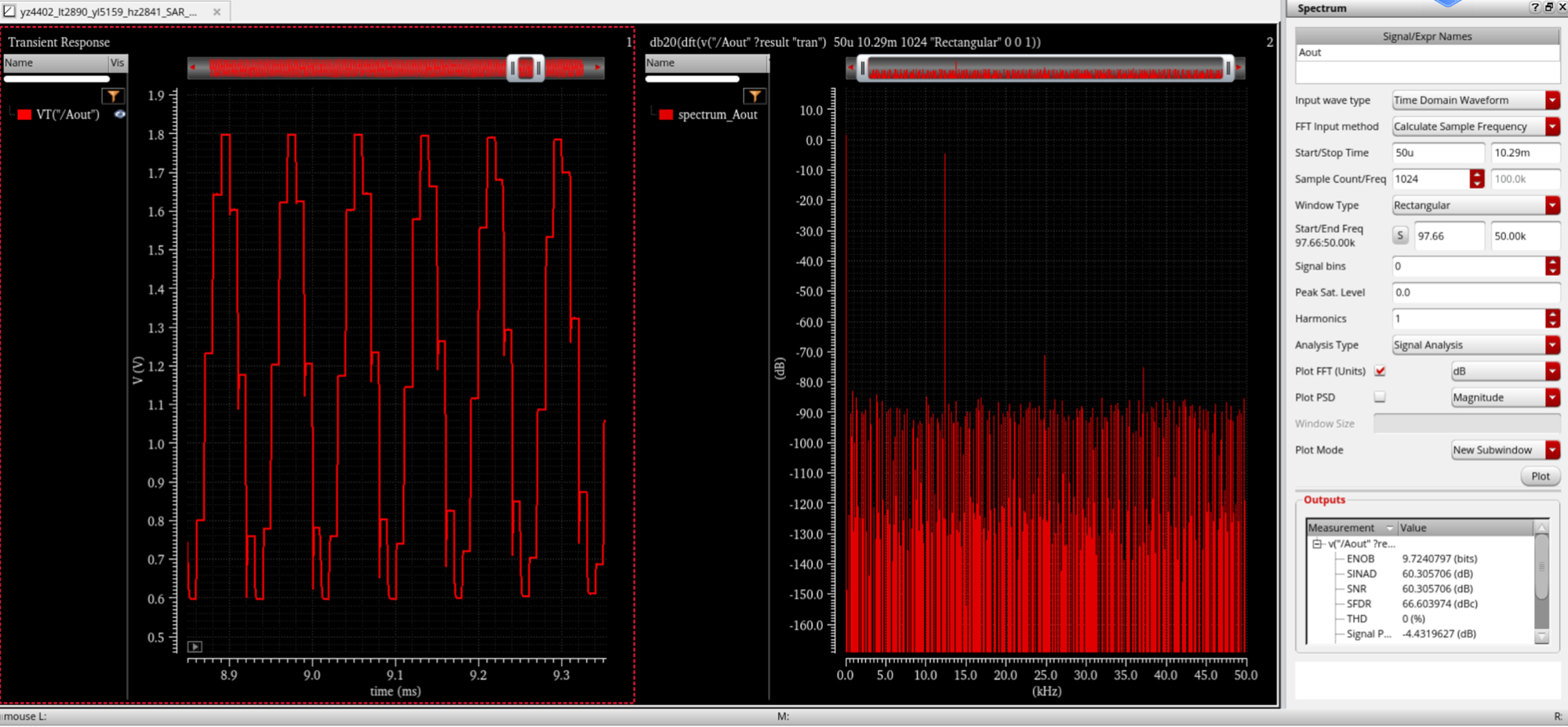
Figure. 2 ENOB Simulation Result
Figure. 3 shows the result of ramp input with full range. We use ideal DAC to transform the 10-bit output back to the analog value and get this result.
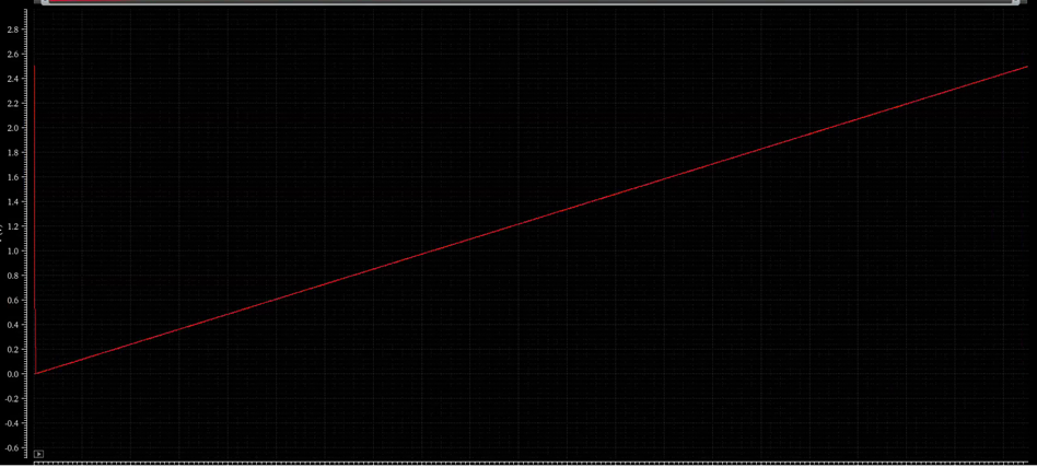
Figure. 3 Ramp Simulation Result
S/H circuit simulation results:
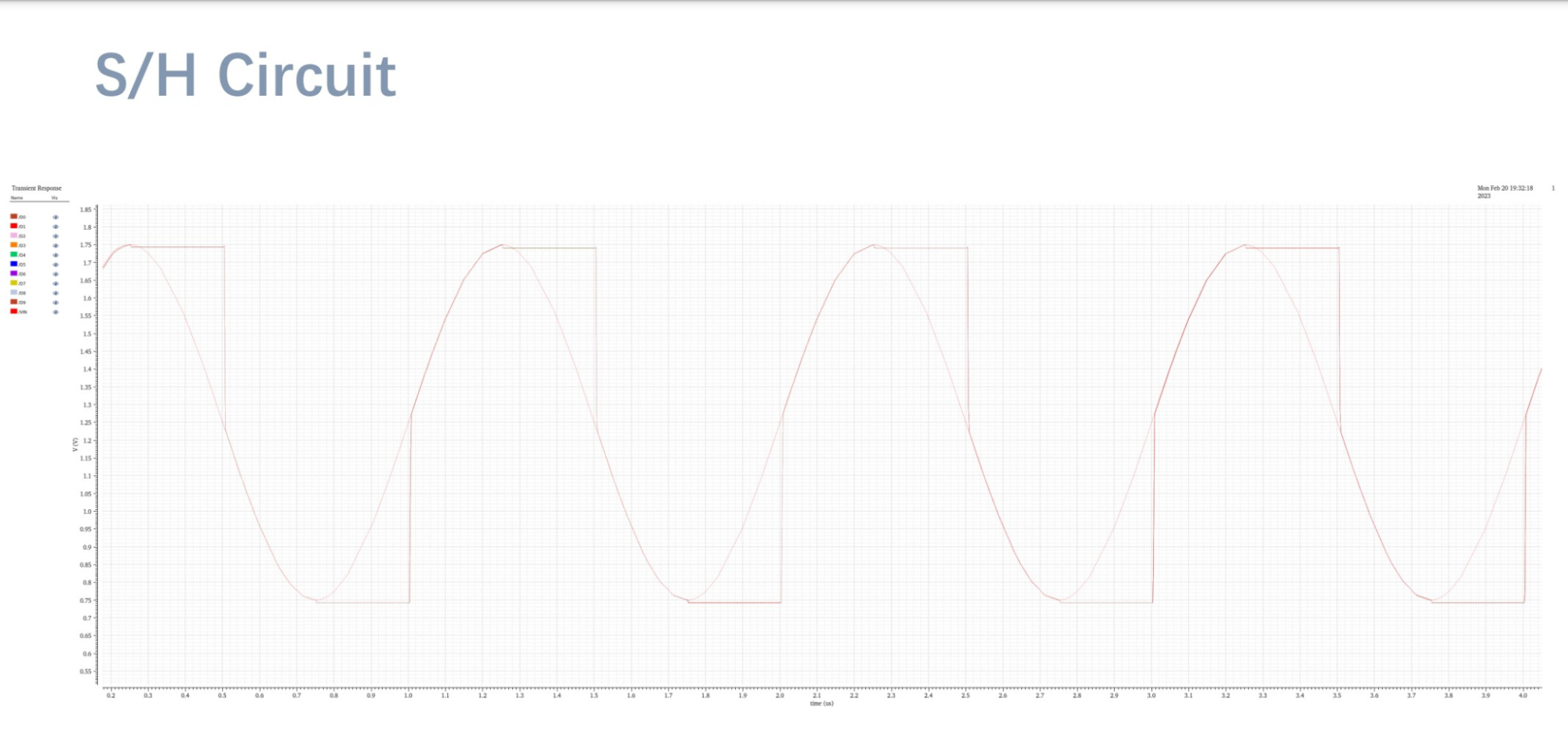
Figure. 4 S/H circuits Simulation Result
Comparator Simulation results: Here is the result of the comparator. This figure happens when two inputs are the same. In this situation, the speed of the comparator is the lowest and it costs 200ps to get the final result.
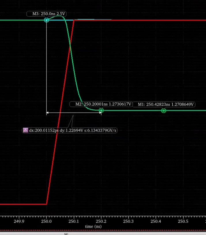
Figure. 5 comparator Simulation Result
SAR Logic Block Simulation results: Here is the simulation result of the SAR logic block. As you can see in the figure, the input of the comparator can be stored in every bit of the register. The value of each bit would not be set to 0 again before the next 1 value for rst input.
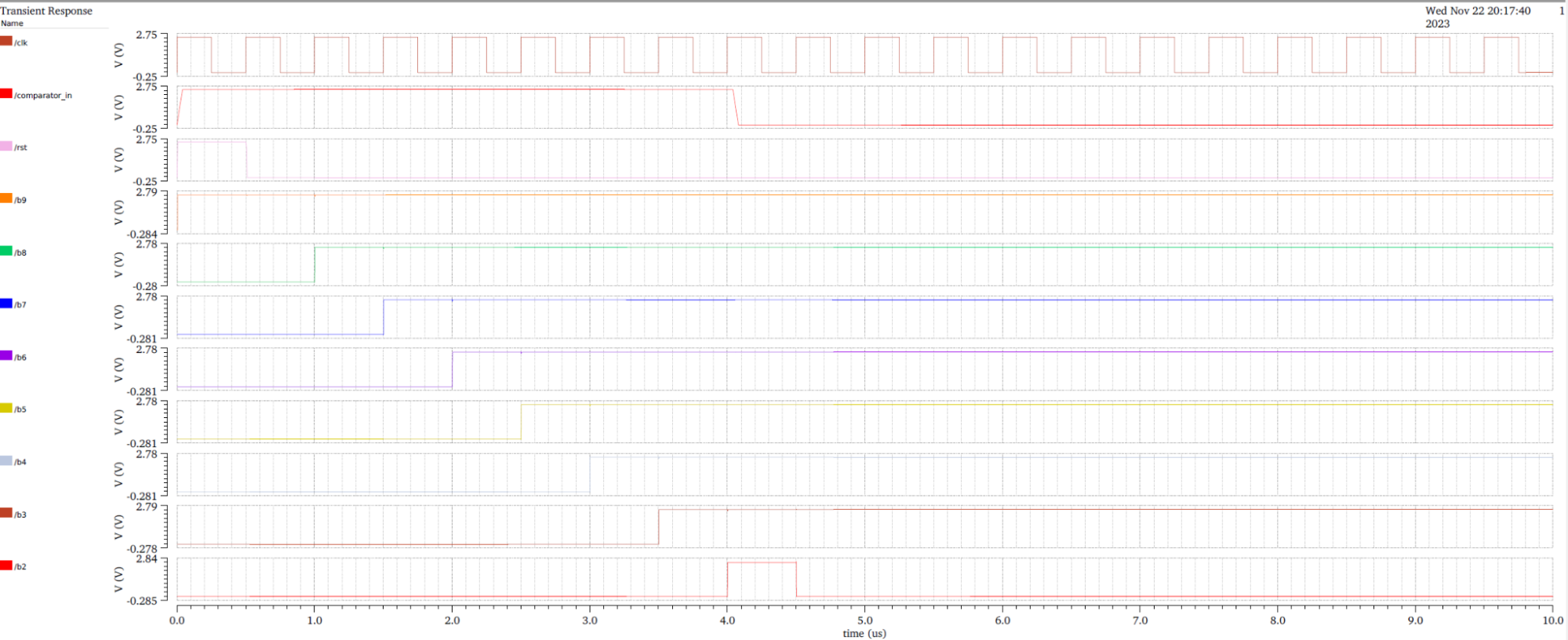
Figure. 6 SAR logic simulation Result
10-bit DAC Simulation Results:
Dynamic simulation testbench
The testing of DAC also adopts the method of coprime input, outputting the input signal to an ideal VerilogA ADC, and then connecting this ADC to our ADC. When outputting, take 4096 valid points, then use the data from these points for DFT analysis, and finally calculate SNDR and ENOB.
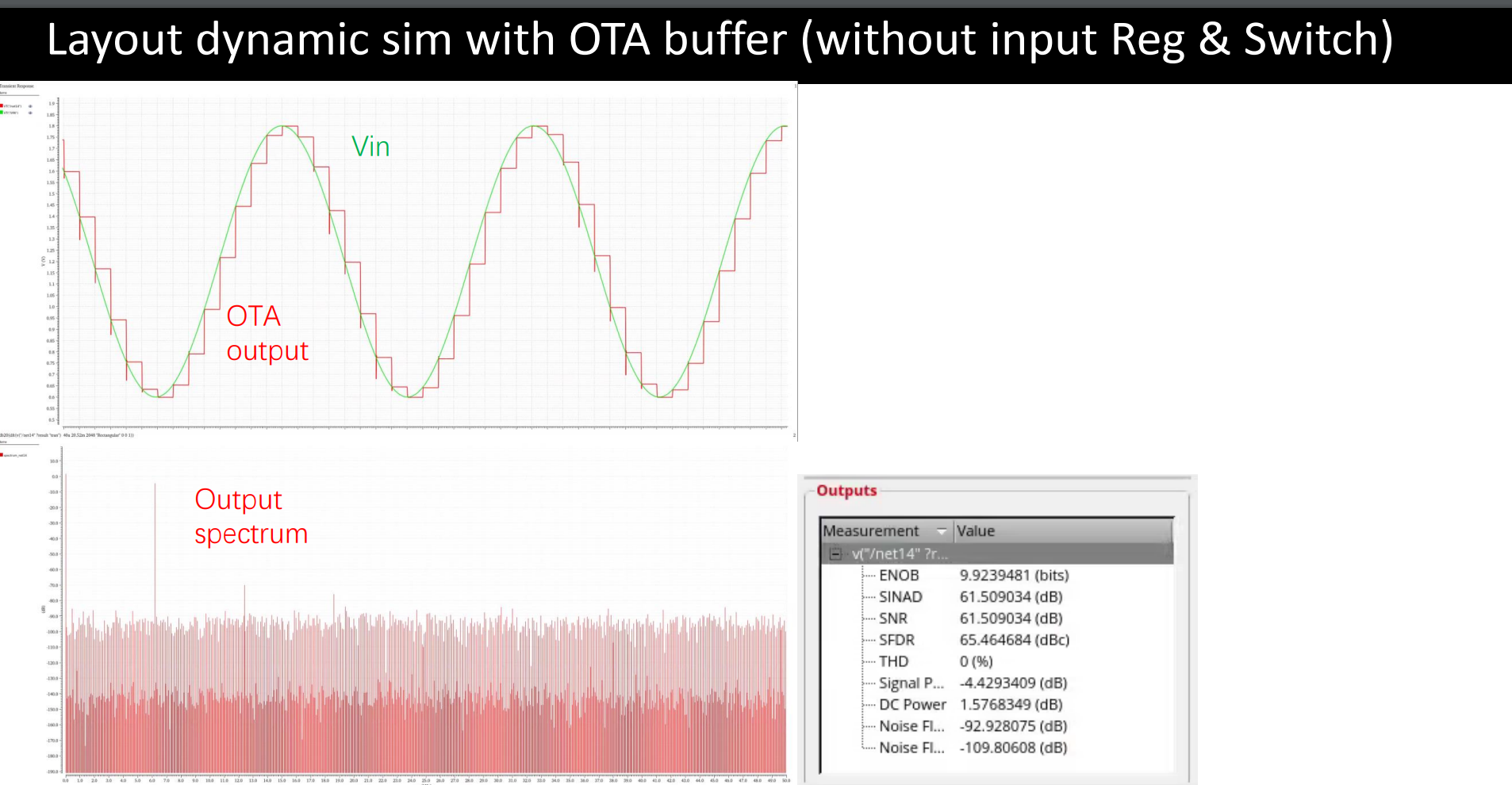
Figure. 7 Dynamic performance simulation Result
Static Performance measurement
The static parameter measurement of a Digital-to-Analog Converter (DAC) is essential for evaluating its performance under stable conditions. Key static parameters include Resolution, which indicates the smallest change in the analog output that the DAC can discern; Differential Non-Linearity (DNL), measuring the deviation between actual and theoretical step outputs; Integral Non-Linearity (INL), which is the maximum deviation from an ideal linear output; Zero Error or Offset Error, the difference between the actual output and theoretical output when the input is zero; Full-Scale Error, the discrepancy at the DAC's maximum input; Gain Error, reflecting the proportional difference between the DAC's output range and the theoretical range. Accurate measurement of these parameters, often requiring precision instruments like high-accuracy voltmeters and oscilloscopes, is crucial for determining the DAC's accuracy and suitability for specific applications.
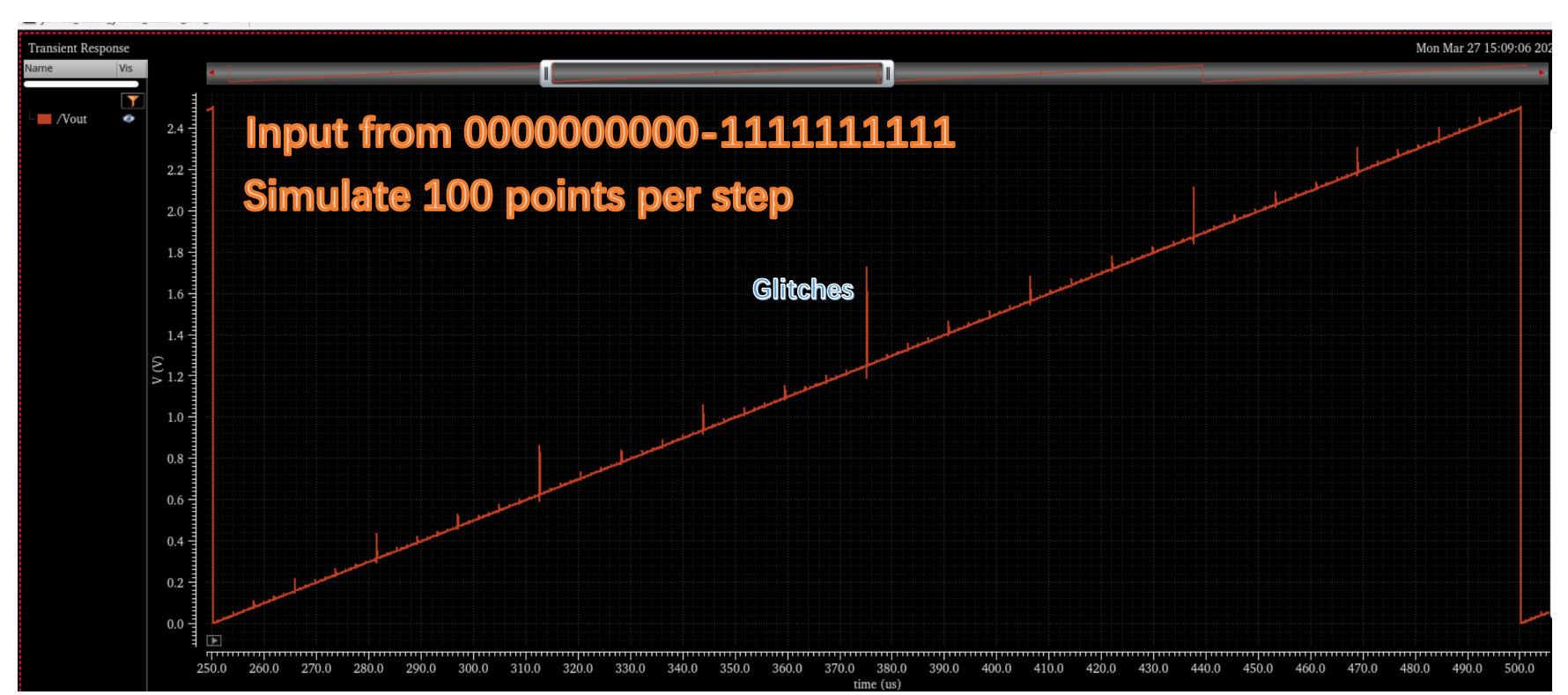
Figure. 8 Static performance simulation Result
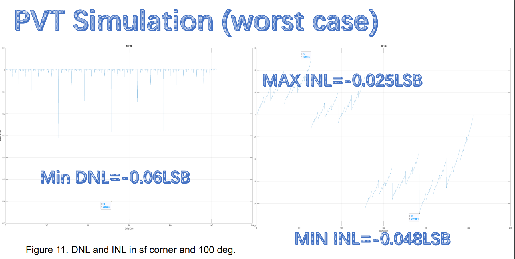
Figure. 9 Plot for DNL/INL measurements
Mismatch evaluation
Steps in Monte Carlo Simulation:
Defining Parameter Variations: First, identify the key parameters affecting DAC performance, such as the values of resistors, capacitors, and their tolerances.
Establishing a Simulation Model: Use Electronic Design Automation (EDA) software to create a circuit model of the DAC. This model should be capable of accepting varied parameter values.
Generating Random Variables: Based on the defined range of parameter variations, generate a series of random parameter values. These values should follow the actual distribution of the parameters, such as normal or uniform distribution.
Performing Multiple Simulations: Conduct multiple simulations of the DAC model using the generated random parameter values. Each simulation uses a different set of parameters to mimic potential scenarios in actual production.
Statistical Analysis: Collect all the results from the simulations and perform statistical analysis. Focus on the distribution of performance parameters (like INL, DNL, gain error, etc.) and the failure rate. Assessing Design Robustness: Evaluate the stability and reliability of the DAC design in the face of random variations during manufacturing, based on the statistical results.