Testing
Characterization
Transistor performance and, as a result, system performance can be significantly affected by variations during the manufacturing process. Therefore, it is necessary to know if the devices on the chip being tested are typical, slow or fast. One way to determine this is to measure the I-V curves for transistors of known sizes on the chip. On our chip, we placed a test NFET on one of the control pins and used this and a PFET being used as a bias transistor to obtain the required I-V curves. By comparing our measurements with simulations, we determined that the chip being tested belonged to the SS (slow-slow) process corner.
Typical operation
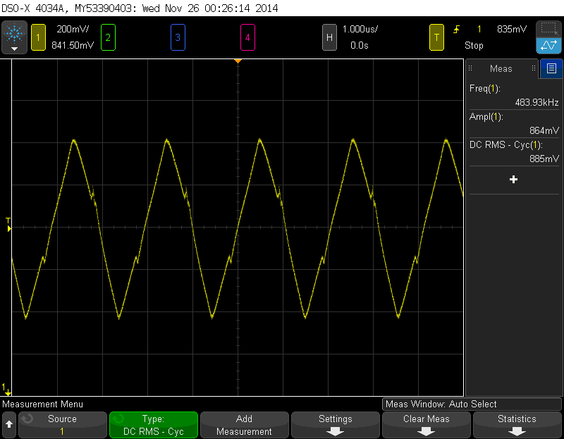
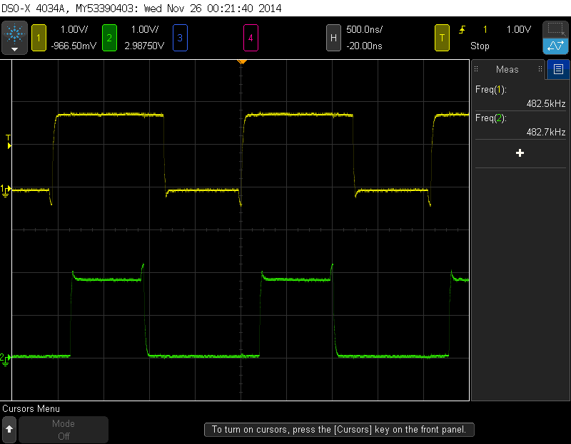
Fundamental to the operation of the class-D amplifier is correct functioning of the PWM block and accurate triangle wave generation is a critical part of this. The triangle wave generator on the chip was designed to produce a triangle wave with a frequency of approximately 500kHz and a peak-to-peak amplitude of 0.9V. The option to supply an external triangle wave was also incorporated into the chip. Figure 1 shows a plot of the triangle wave generated on the chip as measured using an oscilloscope.
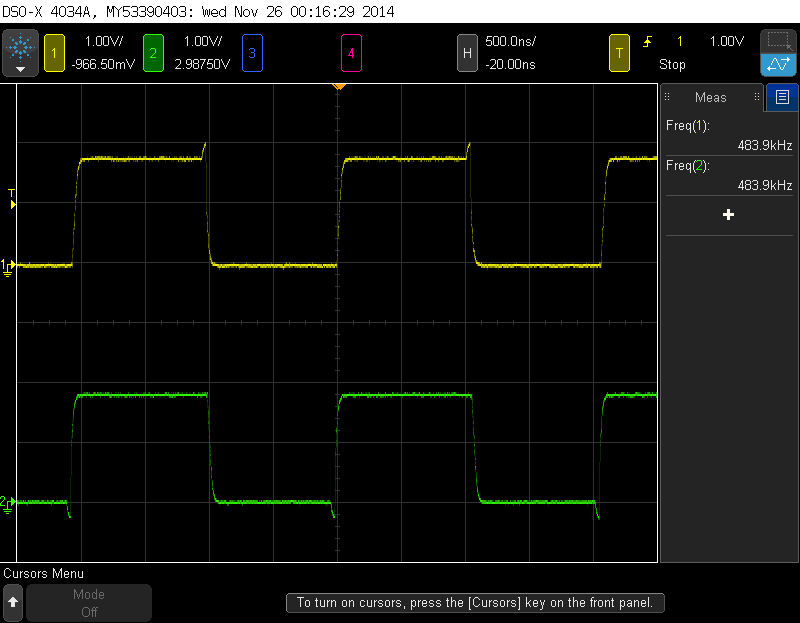
Figures 2 and 3 show plots of the differential output of the chip when no input is applied and when a DC input is applied, respectively. As expected, the duty cycle of the pulses is 50% for no input and changes linearly with the instantaneous amplitude of the input.
Efficiency measurements
One of the most important advantages of the class-D architecture is its high power efficiency compared to amplifiers of other classes. Here, we define the power efficiency ($\eta$) as
\[ \eta = \dfrac{P_{Load}}{P_{Supply}} \]where $P_{Load}$ is the power that is delivered to the load and $P_{Supply}$ is the power drawn from the supply. We can further express these powers as
\[ P_{Load} = \dfrac{V_{RMS,Load}^2}{R_{Load}} \] \[ P_{Supply} = V_{Supply}I_{Supply} \]Of the terms on the RHS of the 2 equations mentioned above, measuring $R_{Load}$ is trivial while $V_{RMS,Load}$ and $V_{Supply}$ can be measured unobtrusively. In order to measure $I_{Supply}$ we introduced a small (0.2$\Omega$) resistance in series with the DVDD source so that the drop across the 0.2$\Omega$ resistor would directly give us the amount of current being drawn from the supply.
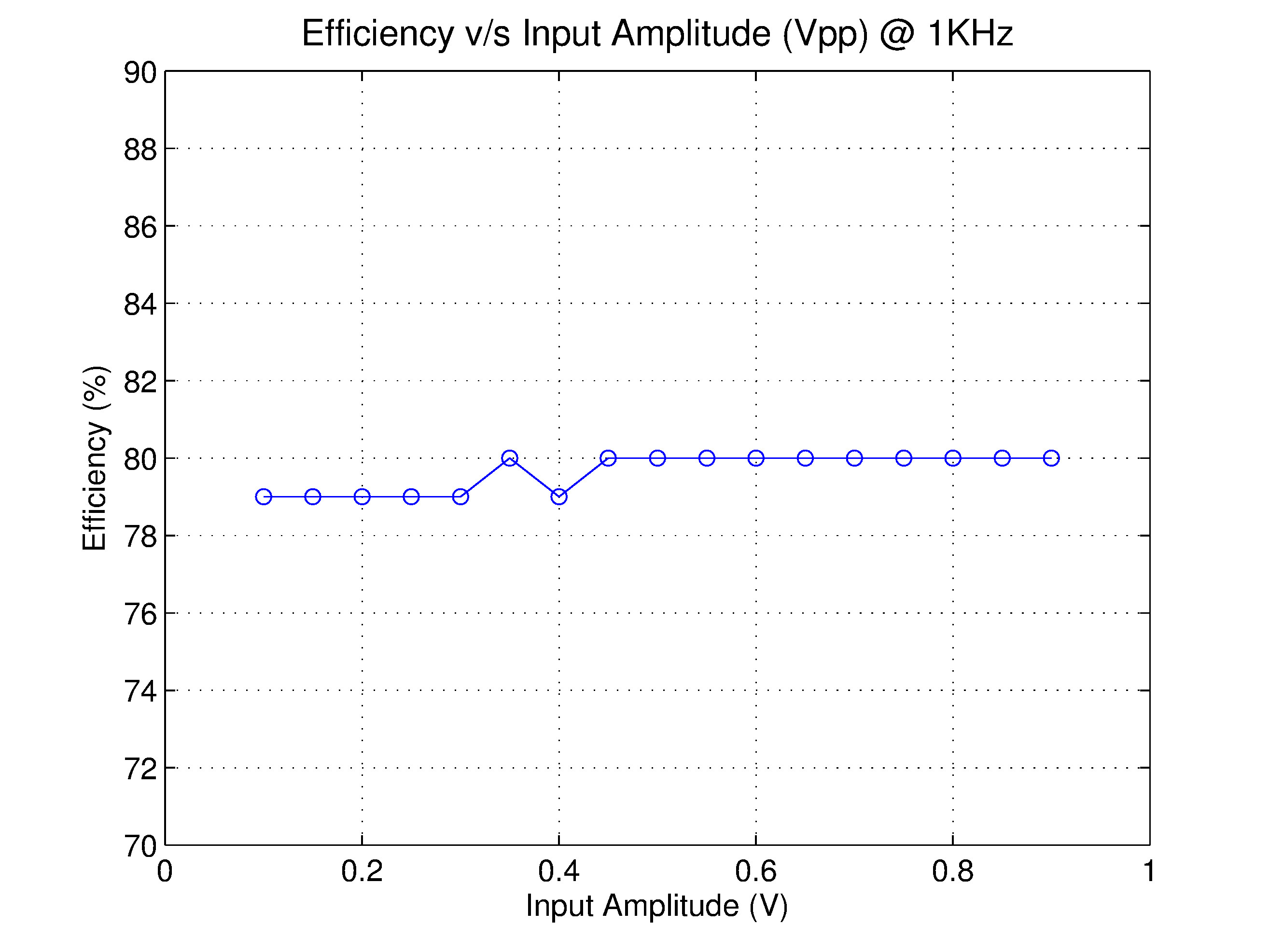
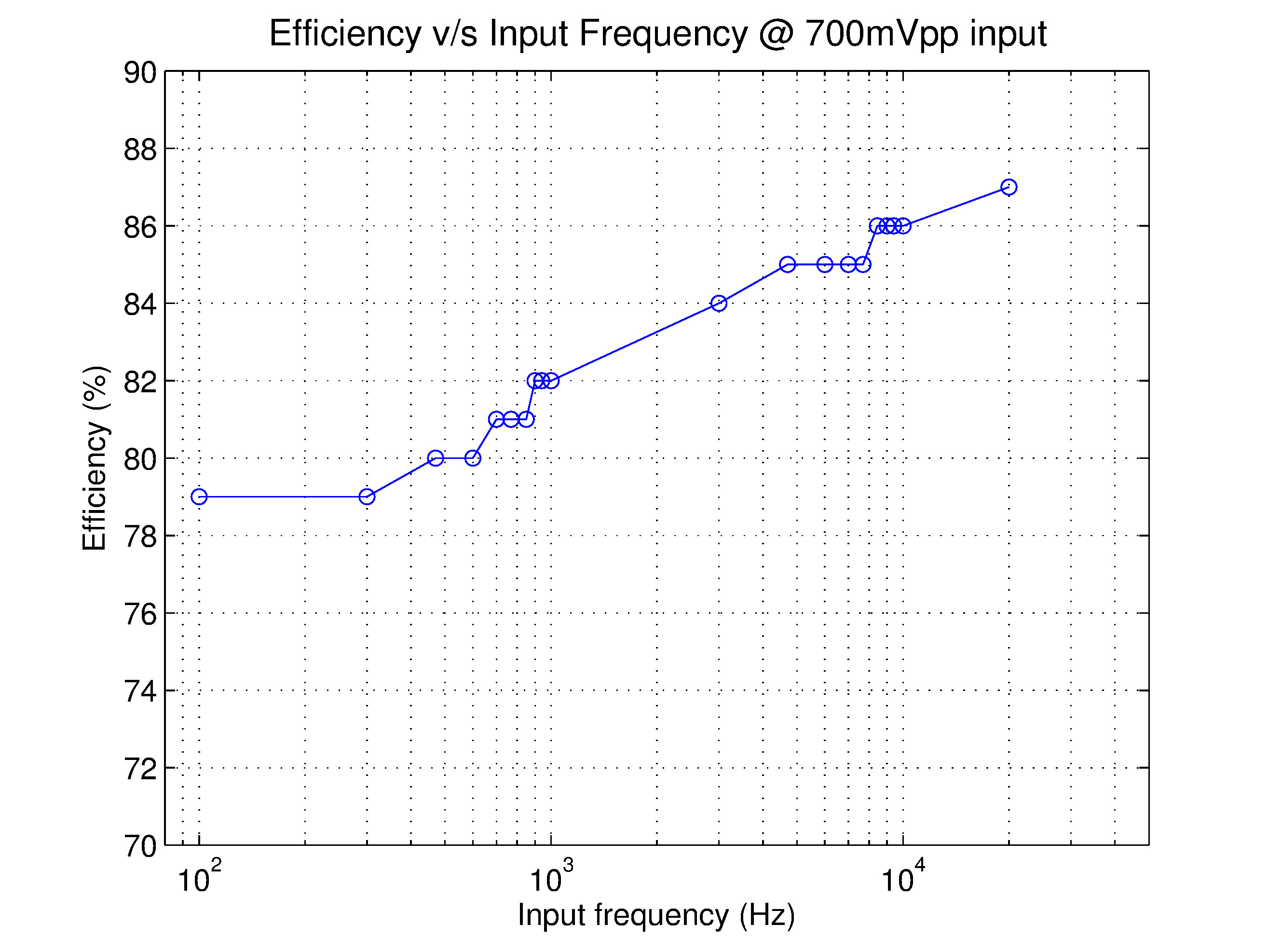
Figures 4 and 5 show the variation of power efficiency with variations in the input signal amplitude and frequency with $R_{Load} = 8.39\Omega$ and $V_{Supply} = $1.8V. In all cases, the efficiency is higher than 78.5% with a maximum efficiency of 86.6% for a 20kHz input. Simulation results at the SS corner indicated that the efficiency should be close to 93%. One of the reasons for the difference could be the 0.2$\Omega$ resistance that we had to introduce in order to be able to measure $I_{Supply}$.
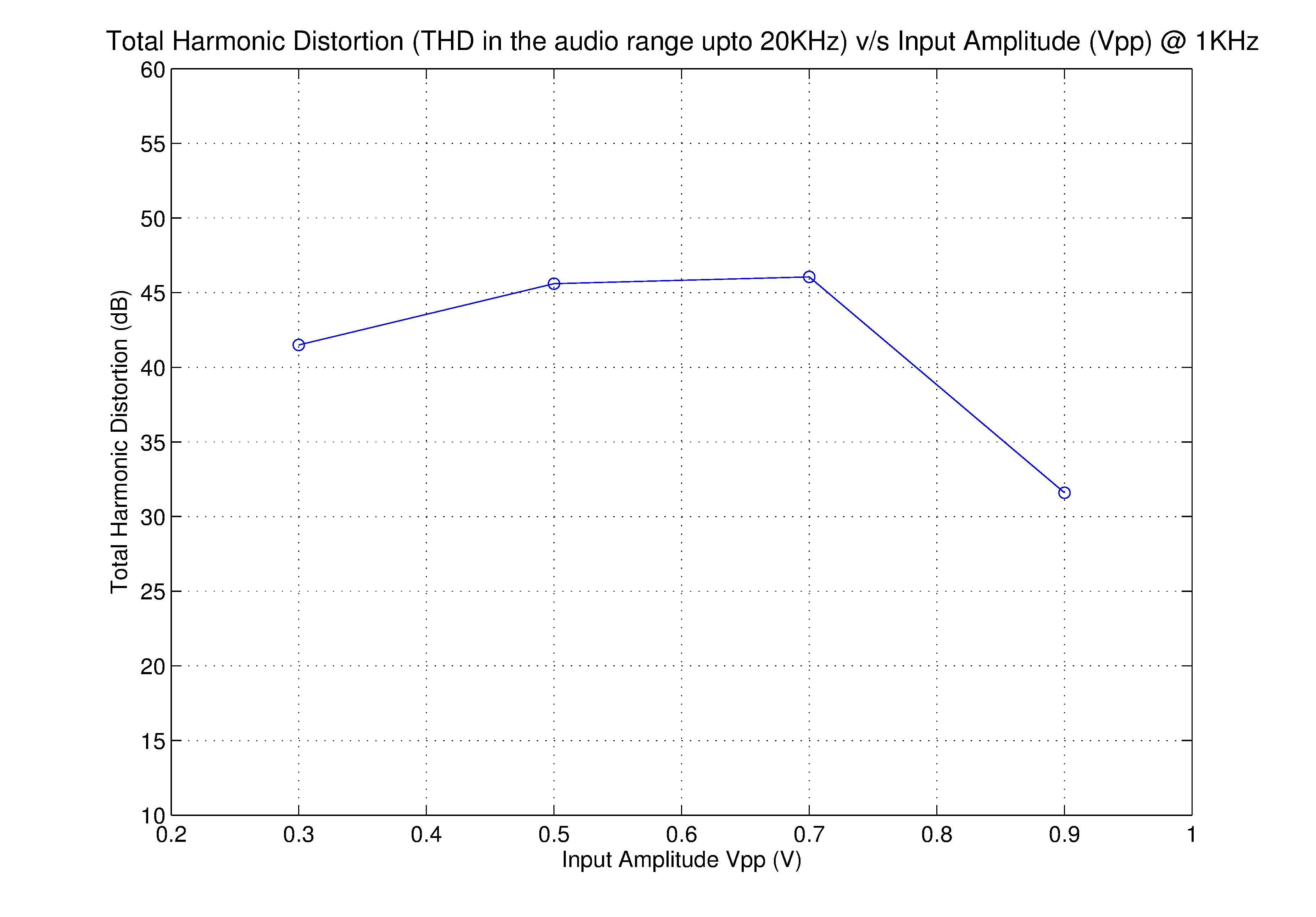
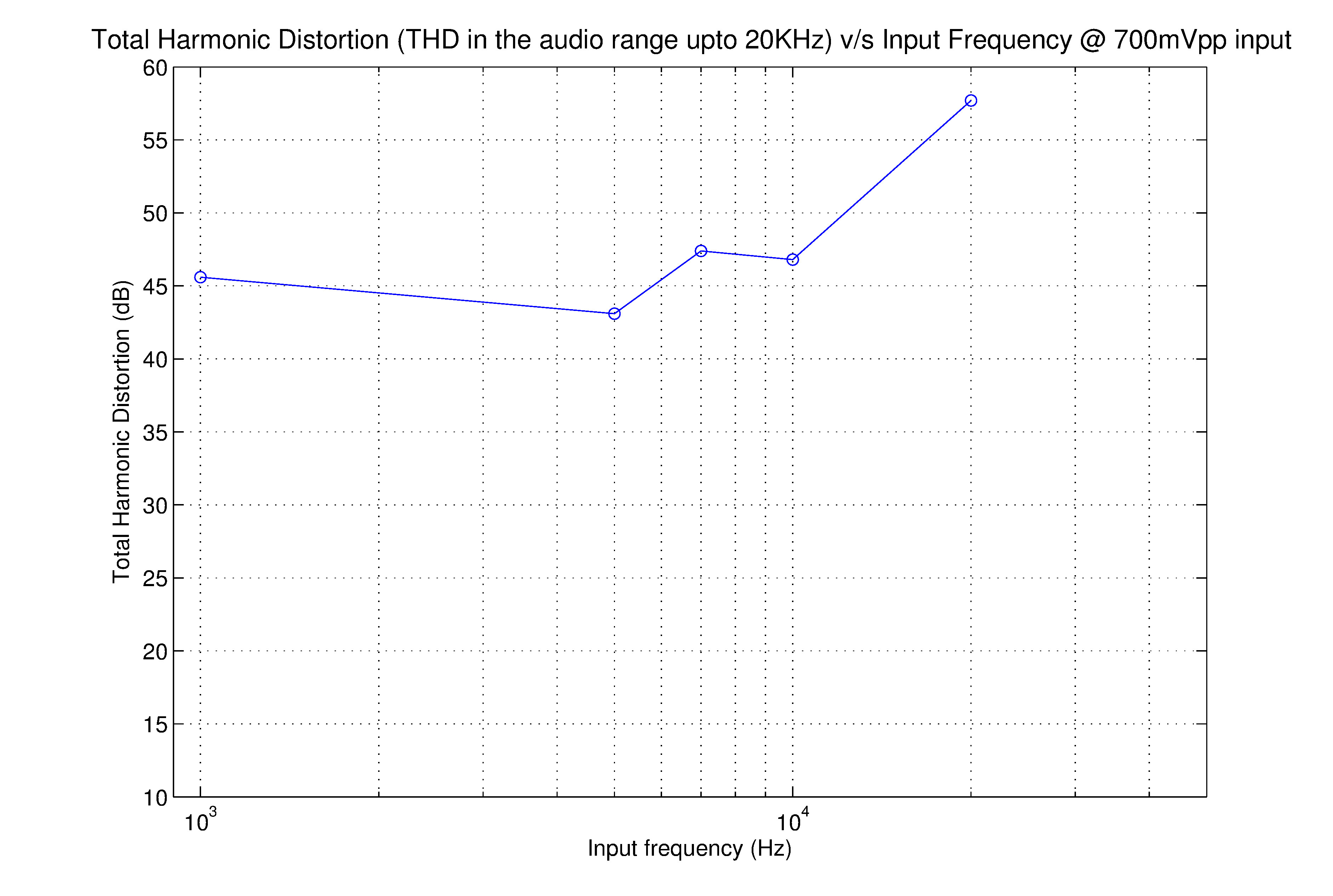
Total Harmonic Distortion (THD) measurements
Distortion is perhaps the most important metric for an audio amplifier. Here, we define the Total Harmonic Distortion (THD) as \[ THD = \dfrac{\sqrt{V_2^2 + V_3^2 + V_4^2 + ...}}{V_1} \] where $V_n$ indicates the RMS voltage of the $n^{\mathrm{th}}$ harmonic of the fundamental frequency. Since this is an audio amplifier, only harmonics within the audio band (20Hz - 20kHz) are included in the THD calculation. Figures 6 and 7 show comparisons of the measured and simulated (for the SS corner) THD for input signals of varying amplitude and frequency. The THD is consistently better than 42dB with a maximum THD 57dB.