3. Part 2: Investigating the Static Graph Expansion Process

3.1. The Model

For this lab, we will be working with the Wall Street Journal corpus. This corpus was created many years ago for a program sponsored by DARPA to spur development of basic LVCSR technology, and this corpus was designed to be about as easy as an LVCSR corpus could be for ASR. The data consists of people reading Wall Street Journal articles into a close-talking microphone in clean conditions; i.e., there is little noise. Since the data is read text, there are few conversational artifacts (such as filled pauses like UH) and it is easy to find relevant language model training data.

We trained an acoustic model on about 10 hours of Wall Street Journal audio data and a smoothed trigram language model on 24M words of WSJ text. The acoustic model is context-dependent; phonetic decision trees were built for each state position (i.e., start, middle, and end) for each of the ~50 phones, yielding about 3*50=150 trees. The trees have a total of about 3000 leaves; i.e., the model contains 3000 GMM's, one for each context-dependent variant of each state for each phone. Each GMM consists of eight Gaussians, so the model contains about 3000*8=24000 Gaussians or prototypes. The model was trained by first training a (1 Gaussian per phone) context-independent phonetic model, using this to seed a (1 Gaussian per leaf) CD phonetic model, and then doing Gaussian splitting until we achieved 8 Gaussians per leaf or GMM. For the front end, we used 13-dimensional MFCC's with delta's and delta-delta's, yielding 3*13=39 dimensional feature vectors. The vocabulary was taken to be the 5000 most frequent words in the LM training data. If this paragraph meant nothing to you, you should probably cut down on the brewski's.

3.2. Graph Expansion Steps

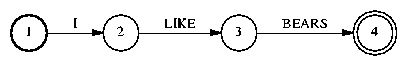
We explain the steps in graph expansion by going through an example. For full-scale decoding, we would start with a word FSM representing a pruned trigram LM; in this example, we start with a word graph wd.fsm containing just a single word sequence:

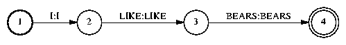
The first thing we do is convert the FSA into an FST:

FsmOp wd.fsm -make-transducer wd2.fsm

resulting in

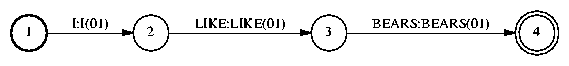
Then, we compose the FST wd2lx.fsm to convert from words to pronunciation variants, or lexemes in IBM terminology:

FsmOp wd2.fsm wd2lx.fsm -compose lx.fsm

In this case, each word has only a single pronunciation variant (e.g., I(01) denotes the first pronunciation variant of the word I), but in general there may be words with multiple pronunciations. This yields

Next, we convert from lexemes to phones:

FsmOp lx.fsm lx2pn.fsm -compose pn.fsm

yielding

Next, we convert from phones to the model level (held in the file md.fsm); this involves applying the phonetic decision trees to find the context-dependent variation at each state position of each phone. We do not explain how we do this since it involves virtual FST's and we don't want to get into this, but the result is

The contents of each decision tree can be found in the file tree.txt. Here is an excerpt of the tree for the feneme AY_1, i.e., the first state of the phone AY:

Tree for feneme AY_1: node 0: quest-P 111[-1] --> true: node 1, false: node 2 quest: | node 1: quest-P 36[-2] --> true: node 3, false: node 4 quest: D$ X node 2: quest-P 66[-1] --> true: node 5, false: node 6 quest: AO AXR ER IY L M N NG OW OY R UH UW W Y node 3: leaf 661 node 4: quest-P 15[-2] --> true: node 7, false: node 8 quest: AXR ER L OW R UW W

Node 0 is the root of the tree. At node 0, question 111 is asked of the phone in position -1 (i.e., the phone to the left); if the question is true, go to node 1, else go to node 2. Question 111 asks whether the given phone belongs to the set {“|”}. By convention, the beginning and ending of utterances are padded with the “-1” phone, or unknown phone. (Recall that the “|” phone is the word boundary phone and is placed at the beginning of each word pronunciation.)

Let us go through a partial example of calculating the leaf number for the first state in the first AY phone in our example. Here, the phone to the left of the first AY is the “|” phone, so the question at the root node is true and we go to node 1. At node 1, we ask about the phone at position -2, or two phones to the left. This is beyond the beginning of the utterance, so this means we use the -1 phone. Since this phone does not belong to the set {D$, X}, the question is false and we go to node 4. The remainder of this example is left as an exercise. Some notes:

• For MERGE nodes, this means that two nodes in the tree were merged into one because they had sufficiently similar output distributions, and you should just go directly to the named node.

• The decision tree used in this example is a left-context decision tree, which means it is only allowed to ask questions across a word boundary for words to the left. (This is kind of halfway between a word-internal and true cross-word decision tree.) That is, if a question is ever asked about a phone position that is beyond the end of the current word, you should pretend the -1 phone is in that position.

Anyway, back to our graph expansion example. In the last step, we expand the FSM to the final HMM, rewriting each model token by the HMM that represents it:

FsmOp md.fsm md2obtr.fsm -compose obtr.fsm

This HMM is too large to display in its entirety, but here is an excerpt:

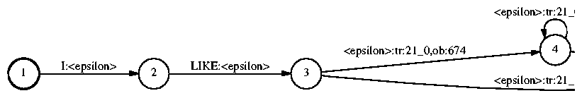
The actual transition probabilities are kept in a separate file, like the file example.tmd. In this file, the first line contains the probabilities corresponding to the tokens tr:0_0 and tr:0_1, respectively, and the last line corresponds to tr:155_0 and tr:155_1. The Gaussian parameters are kept in a file like example.omd, which contains 2-component Gaussian mixtures. In the first part of the file, each line corresponds to a leaf. For each leaf, the index of each Gaussian in the mixture and the mixture weight for that Gaussian is listed. In the latter part of the file, each line corresponds to a Gaussian; the Gaussian indices listed for each leaf are indices into this list of Gaussians. For each Gaussian, the mean and variance for each dimension is listed.

So, this pretty much describes all the data that we need to feed into our decoder. As mentioned before, in real life we begin with a word graph representing an n-gram language model. The LM word graph we used in this lab can be found in lm.fsm.gz; it is a trigram model that has been pruned to about 200k bigrams and 125k trigrams. To look at it, you can use zcat (as it's compressed), e.g.,

zcat lm.fsm.gz | more

The final expanded decoding graph can be found in decode.fsm.gz. It contains about 1.5M states and 4M arcs.

For this part of the lab, you will have to edit some of the FSM's used in our toy example to handle a new word in the vocabulary. In addition, you will need to do some manual decision-tree expansion; see lab4.txt for directions.