<< Back to main page
E6820 Assignment 3
For some reason, this page is a lot longer than the previous pages. So here are links to the appropriate sections:
Reading assignment
Practical assignment
Project
Reading assignment
Paper:
“Construction and evaluation of a robust multifeature speech/music discriminator,” E.
Scheirer and M. Slaney, Proc. ICASSP-97 Munich, 1331-1334.
Summary:
The authors examine many different kinds of features and several
kinds of classification systems in order to discriminate between speech
and music. They managed to build a pretty robust system with
error rates below 2%. Interestingly, when the authors tried to
add a third category of speech with music, their success rate went down
to 65%.
Thoughts:
It's interesting that the authors found that the log of the
features improved the fit of the normal distributions. I wonder
why that is, especially since the authors claim it worked for all 13
features.
I wonder how the CPU Time was really calculated. The authors ran
these tests on workstations, which have operating systems. So,
how did they decide what the CPU usage for a particular task was?
If they just took overall CPU usage, they would have included
things like the operating system's use of the CPU. For that
matter, even supposing that the operating system broke down the CPU
usage, how did it know? Every time you have a context switch,
there's a certain amount of overhead performed on behalf of the
process. Was this counted? There's also the fact that the
cache probably no longer contains stuff of interest to the newly
switched in process. So, initially, the process is going to be
spending time waiting during cache misses. How could any
operating system take that into account?
Back to the top
Practical assignment
I wasn't sure where to put the "assignments" at the end of each section. So, I've put them here. The diary is here.
Assignments:
I. Data and Features:
Here is my matlab code for the assignment. It plays just the sung portions of each sample.
II. Gaussian Mixture Models:
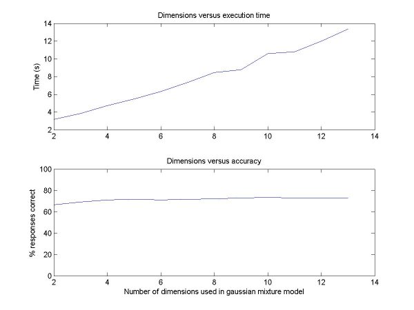
Here
is the code I wrote to produce the plot below. As you can see,
the accuracy didn't go up much at all as the complexity increased, but
the time required for calculations went up almost linearly. I
could have stopped at 4 mfccs quite easily with almost no performance
loss.
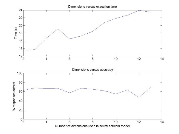
III. Neural Networks
I again had to graph complexity versus accuracy and training time. Here
is the code I wrote to produce the plot below. Oddly enough,
adding extra mfcc dimensions to the neural network did not seem to
improve the neural network's accuracy. It also did not have a
completely predictable effect on the training time. I must
confess that I noticed that the neural network's accuracy varied pretty
wildly when I ran it several times with exactly the same parameters.
It seems possible that for this problem, the Gaussian mixture
model is a better bet because it takes less time and is more reliable.
Matlab diary:
[d,sr] = wavread('music/1.wav');
soundsc(d,sr);
[d,sr] = wavread('music/3.wav');
soundsc(d,sr);
[stt,dur,lab] = textread('labels/3.lab', '%f %f %s','commentstyle','shell');
[stt(1:4),dur(1:4)]
ans =
0 3.3470
3.3470 1.0540
4.4010 2.6190
7.0200 1.2860
lab(1:4)
ans =
'vox'
'mus'
'vox'
'mus'
ll = zeros(length(lab),1);
ll(strmatch('vox',lab)) = 1;
tt = 0.020:0.020:14.980;
lsamp = labsamplabs(tt,[stt,dur],ll);
subplot(311)
plot(tt,lsamp)
axis([0 15 0 1.1])
subplot(312)
specgram(d,512,sr)
soundsc(d,sr)
soundsc(d((1+0*sr):(3.347*sr)),sr)
Warning: Integer operands are required for colon operator when used as index.
cc = mfcc(d,sr,1/0.020);
size(cc)
ans =
13 749
subplot(313)
imagesc(cc)
axis xy
frmpersong = 749;
nsong = 60;
nftrs = 3 * 13;
ftrs = zeros(nsong*frmpersong, nftrs);
for i = 1:60;
[d,sr]=wavread(['music/',num2str(i),'.wav']);
cc = mfcc(d,sr,1/.020);
ftrs((i-1)*frmpersong+[1:frmpersong],:) = [cc', deltas(cc)', deltas(deltas(cc,5),5)'];
end
labs = zeros(nsong*frmpersong, 1);
for i = 1:60;
[stt,dur,lab] = textread(['labels/',num2str(i),'.lab'], '%f %f %s','commentstyle','shell');
ll = zeros(length(lab),1);
ll(strmatch('vox',lab)) = 1;
lsamp = labsamplabs(tt,[stt,dur],ll);
labs((i-1)*frmpersong+[1:frmpersong])=lsamp;
end
size(labs)
ans =
44940 1
size(ftrs)
ans =
44940 39
mean(ftrs)
ans =
Columns 1 through 7
-14.4471 0.3160
-0.1459 -0.0065 -0.1342
-0.0503 -0.0562
Columns 8 through 14
-0.0376 -0.0295
-0.0271 -0.0001 -0.0596
-0.0061 -0.0114
Columns 15 through 21
-0.0151 0.0057
0.0040 0.0019 -0.0086
0.0056 0.0122
Columns 22 through 28
0.0020 0.0013
0.0013 -0.0006 0.0043
0.0066 0.0025
Columns 29 through 35
0.0044 0.0013
0.0004 0.0004
0.0013 0.0017 -0.0024
Columns 36 through 39
-0.0001 0.0015 0.0018 -0.0025
mean(labs)
ans =
0.4740
ddS = ftrs(labs==1,:);
ddM = ftrs(labs==0,:);
subplot(221)
plot(ddM(:,1),ddM(:,2),'.b',ddS(:,1),ddS(:,2),'.r')
subplot(222)
plot(ddS(:,1),ddS(:,2),'.r',ddM(:,1),ddM(:,2),'.b')
ndim = 2;
nmix = 5;
gmS = gmm(ndim,nmix,'diag');
gmM = gmm(ndim,nmix,'diag');
options = foptions;
options(14) = 5;
gmS = gmminit(gmS, ddS(:,1:2), options);
Warning: Maximum number of iterations has been exceeded
gmM = gmminit(gmM, ddM(:,1:2), options);
Warning: Maximum number of iterations has been exceeded
options = zeros(1, 18);
options(14) = 20;
gmS = gmmem(gmS, ddS(:,1:2), options);
Warning: Maximum number of iterations has been exceeded
gmM = gmmem(gmM, ddM(:,1:2), options);
Warning: Maximum number of iterations has been exceeded
xx = linspace(-28,-8);
yy = linspace(-5,5);
[x,y] = meshgrid(xx,yy);
ppS = gmmprob(gmS, [x(:),y(:)]);
ppS = reshape(ppS, 100, 100);
subplot(223)
imagesc(xx,yy,ppS)
axis xy
ppM = gmmprob(gmM, [x(:),y(:)]);
ppM = reshape(ppM, 100, 100);
subplot(224)
imagesc(xx,yy,ppM)
axis xy
subplot(111)
surf(xx,yy,ppM, 0*ppM)
hold on
surf(xx,yy,ppS, 1+0*ppS)
lS = gmmprob(gmS, ftrs(:,[1 2]));
lM = gmmprob(gmM, ftrs(:,[1 2]));
llrSM = log(lS./lM);
mean( (llrSM > 0) == labs)
ans =
0.6661
[M0,M1] = traingmms(ftrs(:,[1 2]), labs, 5);
Warning: Maximum number of iterations has been exceeded
Warning: Maximum number of iterations has been exceeded
Warning: Maximum number of iterations has been exceeded
Warning: Maximum number of iterations has been exceeded
Accuracy on training data = 66.3%
Elapsed time = 2.5 secs
[M0,M1] = traingmms(ftrs(:,[1 2]), labs, 10);
Warning: Maximum number of iterations has been exceeded
Warning: Maximum number of iterations has been exceeded
Warning: Maximum number of iterations has been exceeded
Warning: Maximum number of iterations has been exceeded
Accuracy on training data = 66.7%
Elapsed time = 4.657 secs
options = zeros(1,18);
options(9) = 1;
options(14) = 10;
nhid = 5;
nout = 1;
alpha = 0.2;
ndim = 2;
net = mlp(ndim, nhid, nout, 'logistic', alpha);
net = netopt(net, options, ftrs(:,1:2), labs, 'quasinew');
Checking gradient ...
analytic diffs delta
1.0e+003 *
-0.0286 -0.0286 0.0000
-0.0007 -0.0007 -0.0000
0.0010 0.0010 -0.0000
-0.0000 -0.0000 0.0000
1.7724 1.7724 -0.0000
0.0894 0.0894 -0.0000
-0.0003 -0.0003 0.0000
-0.0001 -0.0001 0.0000
0.0001 0.0001 0.0000
-0.0000 -0.0000 0.0000
0.0025 0.0025 0.0000
-0.0001 -0.0001 -0.0000
-0.1487 -0.1487 -0.0000
-0.0000 -0.0000 -0.0000
0.0001 0.0001 -0.0000
8.0081 8.0081 -0.0000
8.0114 8.0114 -0.0000
7.6842 7.6842 -0.0000
-8.0115 -8.0115 0.0000
8.0114 8.0114 -0.0000
-8.0115 -8.0115 0.0000
Warning: Maximum number of iterations has been exceeded in quasinew
nno = mlpfwd(net, [x(:),y(:)]);
nno = reshape(nno, 100, 100);
subplot(221)
imagesc(xx,yy,nno)
axis xy
subplot(222)
imagesc(xx,yy,log(ppS./ppM))
axis xy
subplot(223)
imagesc(xx,yy,nno>0.5);
axis xy
subplot(224
??? subplot(224
|
Error: ")" expected, "end of line" found.
subplot(224)
imagesc(xx,yy,log(ppS./ppM)>0)
axis xy
nnd = mlpfwd(net, ftrs(:,[1 2]));
mean( (nnd>0.5) == labs)
ans =
0.6333
net = trainnns(ftrs(:,[1 2]), labs, 5, 10);
Checking gradient ...
analytic diffs delta
1.0e+003 *
-0.0003 -0.0003 -0.0000
0.0001 0.0001 0.0000
-0.0208 -0.0208 0.0000
-0.0013 -0.0013 -0.0000
-0.5552 -0.5552 -0.0000
-0.0716 -0.0716 -0.0000
0.0001 0.0001 -0.0000
-0.0001 -0.0001 0.0000
-0.1515 -0.1515 0.0000
0.0308 0.0308 0.0000
-0.0001 -0.0001 -0.0000
0.0020 0.0020 0.0000
0.0526 0.0526 -0.0000
-0.0002 -0.0002 0.0000
0.0082 0.0082 0.0000
-1.0855 -1.0855 -0.0000
-1.0839 -1.0839 -0.0000
0.8255 0.8255 0.0000
-1.0853 -1.0853 -0.0000
-1.1682 -1.1682 0.0000
-1.0854 -1.0854 -0.0000
Warning: Maximum number of iterations has been exceeded in quasinew
Accuracy on training data = 66.1%
Elapsed time = 12.172 secs
diary off
Back to the top
Project
Work on the project can be found on my project page here.
Back to the top
Christine Smit
