 EE6850
Home |Previsous: System | Up:
Intro |Next: Decision
EE6850
Home |Previsous: System | Up:
Intro |Next: Decision
This section will describe:
2 kinds of features -- color histogram and edge histogram;
3 kinds of distance measures -- L2 distance, cosine distance, histogram intersection.
Preprocessing:
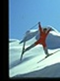
Many images in the database has black boundaries (see figure 1). These boundaries are perceptually insignificant(usually they are not even noticed as part of the image content) and yet they may significantly affect our feature values (e.g. it produces strong fake edges).
Hence, only the center part (5%~95% in each dimension) of every image is used for feature calculation.
Figure 1. Black boundary at the lower left corner of image No.103Color Histogram[1]
MPEG-7 256-bin HSV histogram for the entire image.
1) Input image color space: RGB, convert to HSV space use algorithms presented in [2]. Here the hue value of "greys" (where R=G=B) are set to 0 instead of leaving it undefined, for the convinience of computation.
2) Then, each color component is unifromly quantized: H -- 16 bins; S -- 4 bins; V -- 4 bins.
3) Finally, concatenate this 16x4x4 histogram and we get a 256-dimensional vector.Edge Histogram
Here a 4-bin edgehistogram is used to represent the strength of edge in 0, pi/4, pi/2, 3*pi/4 directions.
1 ) Image gradients Gx and Gy are computed using sobel operators;
sobel_y = [1 0 -1; 2 0 -2; 1 0 -1];
sobel_x = [1 2 1; 0 0 0; -1 -2 -1];
2) Compute edgemap with sobel operator using matlab function edge.m, the cut-off percentage is determined using an RMS estimate of image noise;
3) For each edge pixel, compute the edge direction theta = atan(Gy/gx);
4)Edge direction theta is then unifromly quantized to 4 bins(0, +/-45, 90 degrees) using the decision values +/- 22.5, +/-67.5 degrees.
5) Edge histogram is then normalized w.r.t. the image size, i.e. each bin value represents the percentage of a certain edge direction in an image.Here we also compared this simple edge histogram with a variant of MPEG-7 edge histogram[1], outlined as:
1) Use 5 kinds of 2x2 operators(see figure 2) to compute gradient in 5 directions: 0, +/-45, 90, and isotropic.
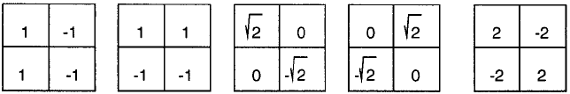
Figure 2. MEPEG-7 Edge Filters, left to right: 0, 90, -45, 45 degree, and isotropic
2) Threshold the gradient values to get # of edge points in each direction, thus form a 5-bin histogram. The thresold used for all 5 operators is 100;
3) We did not segment the image into 4x4 subimages and compute the edge histogram for each of them because our images are already small (192x128).We choose not to use MPEG-7 edge histogram for this HW, bacuase in this particular implementation for our HW dataset, our 4-bin simple edge histogram outperform MPEG-7 edge histogram (see an example
).
Possible reasones are:
1) The sobel operators used here is more robust to noise than the the recommended 2x2 operators because it has larger(3x3) support;
2) Thresholds in mpeg-7 implementation are hard to determine, and its performance vary across images. This also leads to multiple classification of a single edge point, and the "isotropic" class often includes edges in almost all other directions.
3) The performance of mpeg-7 edge histogram could improve if also employing some adaptive thresholding.Taking edge features into account does outperform queries using color features only, see an example
Distance Measures
We tried 3 kinds of histogram distance measures for a histogram H(i), i=1,2,.., N1) L-2 Distance
Defined as:, this metric is uniform in terms of the Eucledian distance between vectors in feature space, but the vectors are not normalized to unit length (infact, they are on a hyperlane if the histogram is normalized).
2) Cosine Distance
If we normailze all vectors to unit length, and look at the angle between them, we have cosine distance, defined as:
, this is different from a common definition[3]
because the former is more uniform in terms of the angle between the two vectors. For example, 45 degree will be in a middle position between 0~1 in the former, but 60 degree will be in the middle for the latter.
This will not cause a problem if a single feature is used, since all the functions are monotonic in valid range; but problem may occur if we wish to combine 2 or more different metrics.3) Histogram Intersection
Defined as:
The denominator term is needed for non-normalized histogram features (for example, edge histogram).
Metric used in our experiment:
1) Histogram intersection works slightly better than the other two kinds of distance in the experiments, see an example
2) Most of our results are calculated using histogram intersection.[1] Manjunath, B.S.; Ohm, J.-R.; Vasudevan, V.V.; Yamada, A., "Color and texture descriptors", IEEE Trans. CSVT, Volume: 11 Issue: 6 , Page(s): 703 -715, June 2001 (section III.B)
[2] Alvy Ray Smith, "Color Gamut Transform Pairs", SIGGRAPH '78
[3] John R. Smith, "Integrated Spatial and Feature Image Systems: Retrieval, Analysis and Compression", Ph.D. thesis, Columbia Univ. 1997 (section 4.3.1)