EE 4830 Spring 2009

HW #3

Due: March 30th, Monday

(1) KL Transform with hand-written digits (50%)

Shown below is a random sample of the USPS hand-written digit dataset. The task for this problem is to experiment with linear projections and make sense out of them in low dimensions.

* USPS data from http://www.cs.toronto.edu/~roweis/data.html

Read in the USPS data (usps_digits.mat), each cell in the variable "usps" contain 1100 instances of one digit. Visualize, say the first 400 instances of digit "2" with vis_digits.m, as follows:

>> clear all
>> load usps_digits
>> whos
  Name      Size    Bytes    Class    Attributes
  usps      1x10    2816600  cell

>> size(usps{2})
ans =
          16          16        1100

>> vis_digits(usps{2}, 1:400);

Work with the following two subset of the data:
(1a) the first 250 vectors of digits "3", "6" and "9" (750 digits in total)
(1b) the first 750 vectors of digit "6"

(1.1) (10%) Random projection. Treat each 16-by-16 digit image as a 256-dimensional column vector, generate a 2-dimensional random project matrix R using RandOrthMat.m (from matlab central) as shown below. Poject data (1a) and (1b) into the two dimensions defined by matrix R. Plot the two 750-point data sets (with different colors or symbols for different digits) onto the x-y plane (one dataset per figure). Compute the data covariance matrix for (1a) and (1b) in the projected space.

>> R = randorthmat(256, 2)';
%%  verify that R is orthonomal 
>> diag(R*R')

(1.2) (15%) Projection with KL-transform. Compute the KL-transform of dataset (1a) and (1b). Project the data of into two dimensions with the KL-transform basis and plot them in the x-y plane as in (1.1). Compute the data energy (variances) in each of the two dimensions and compare the variance values with those in (1.1), also visually compare the two graphs.

(1.3) (10%) Visualize the KL transform basis.
Resize the first two eigen vectors of dataset (1a) and (1b) into a 16-by-16 matrix each, display them as images. Submit these four "basis images" and explain what you see.

(1.4) (15%) Examine the signal energy distribution in transform coefficients.
For a unitary transform A, the "energy coverage" C(d) at dimension d can be defined as the percentage of signal energy that can be recovered using no more than d transform coefficients. Plot on the same figure the d vs. C(d) curve for dataset (1a) with the following transforms, comment on what you see.

(2) A rotational motion blur filter. (20%)
G&W book problem 5.19 (in both 2nd and 3rd edition).
Write or sketch the filter causing the rotational blur in an appropriate coordinate space, explain how you would "undo" the rotational motion blur of a space craft as described in the problem.

(3) Image retoration (30%)

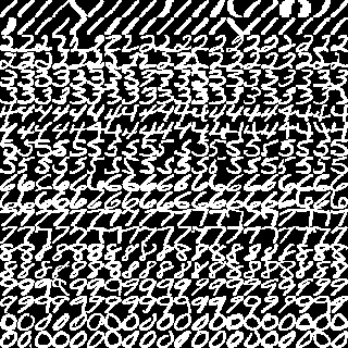
urbanblur.png is a blurred version urban0.png. Use Wiener filter to restore the blurred image.

Write out the transfer function of the filter being used. Guess and try a few filter parameters, present the resulting pictures, compute their mean-square-error from the original image, and discuss what you see.

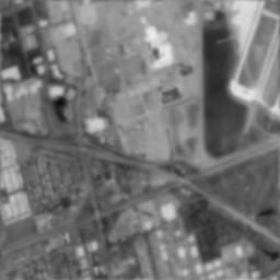urbanblur.png	urban0.png