pout.png
(1) Laplacian and Unsharp Masking (25%)
Show that subtracting the Laplacian from an image is proportional to unsharp masking. Use the definition for the Laplacian in the discrete case to derive the equivalence relation, constant weighting factors should not affect your conclusion.
(2) Spatial processing for photo enhancement (25%)
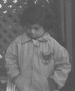
(2.1) Implement a function for histogram equalization and use it on "pout.png"
below (do not use the histeq() function)
(2.1.1) [10%] Include your source code and the equalized image. Plot the intensity
transformation function u vs. v obtained from the equalization
function.
Compare the results with histeq() in matlab (if you have image processing toolbox).
(2.1.2) [5%] Experiment with contrast stretching with matlab or in an image
editing software (e.g. GIMP, or one that you prefer) comment on the outcome
in comparison with (2.1.1).
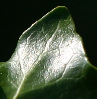
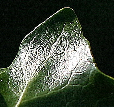
(2.2) [10%] Sharpen the input image leaf.jpg below. Possible techniques include
contrast stretching, histogram equalization, and other matlab functions such as fspecial, filter2, etc.
Compare your result with those from an image processing software, and the authors' result shown on the right. Comment on the techniques you tried and
their visual effects.
(2.3) [5% bonus] Take an image (photo you took, medical image, or images from
the web), enhance it with spatial processing.
Submit the "before" and "after" (as in 2.2), discuss the
steps and why it looks better.
the images can be downloaded as a zip pack here.
|
|
|
pout.png
|
|
|
|
| leaf.jpg | leaf (enhanced) |
image credit: matlab image processing toolbox, and http://flickr.com/photos/greywulf/35159743
(3) High-frequency emphasis and histogram equalization (25%)
G&W 3rd Ed: Problem 4.39 page 310
or G&W 2nd Ed: Problem 4.17 page 217
(4) DFT and DCT on images (25%)
In this homework, we want to analyze the energy distributions of different types of images. A zip pack of the four images used for experiments can be downloaded here.
(4.1) [15%] Convert the input M-by-N color image to the grayscale format. Plot the 2-D log magnitude of the 2D DFT and DCT of the grayscale image, with center shifted. Visually compare and comment on the similarity/differences among the images using the two transforms.
(4.2) [10%] Apply the truncation windows discussed in the class to keep 25%
and 6.25% (1/4 and 1/16) of the DFT and DCT coefficients, i.e. two differen
ratios for each transform. This truncation is done by keeping the coefficients
of the lowest frequencies (those within a centered smaller rectangle of (M/2)x(N/2)
and (M/4)x(N/4) on the shifted FFT, respectively), and setting the coefficients outside this rectangle to zero. Apply the 2D inverse
DFT and inverse DCT
to reconstruct the image for each of the truncated spectra. Compute the Signal-to-Noise-Ratio
(SNR) value for each of the reconstructed images. Plot the reconstructed images
visually examine and comment on the effects of truncation.
 |
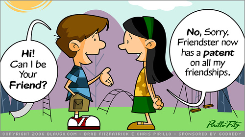 |
| field of dreams ... ** | friendster or foe ** |
 |
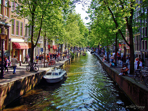 |
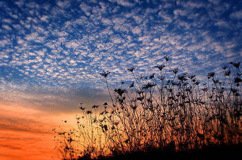
| a queen anne kind of sky** | amsterdam |
* from Flickr URLs below, reused
with the creative commons
license
"friendster or foe" http://www.flickr.com/photos/lockergnome/187472384/
"field of dreams" http://www.flickr.com/photos/ucumari/479872009/
"a queen anne kind of sky" http://flickr.com/photos/jamesjordan/1903863438/
"amsterdam" http://www.flickr.com/photos/claudio_ar/2644023246/