Synthesizing a Guitar Using Physical Modeling Techniques

Introduction

Time Domain Digital Waveguide Modeling

The vibration of a string can be modeled simply using a digital waveguide. This consists of two delay lines representing two travelling waves moving in opposite directions. By summing the values at a certain location along the delay lines at every timestep, we obtain a waveform. This waveform is the sound heard with the pickup point placed at that relative location. The delay elements are initialized with a shape corresponding to the initial displacement of the string. For simplicity a triangular wave is used even though in reality the initial displacement of a plucked string will not be shaped exactly like a triangle. Simply using two delay lines in this fashion would require arbitrarily long delay lines depending on the length of the desired output. By feeding the delay lines into each other a system can be created that can run for an arbitrary amount of time using fixed size delay elements.

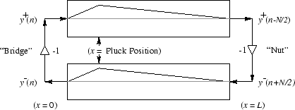
Figure 1: Digital waveguide with initial conditions of delay lines set to triangular waves.

In modeling a guitar it is important to note that the ends of the string are rigidly terminated, so the waves reflect at either end of the string. This effect can be modelled by negating each sample after it reaches the end of a delay line, before feeding it into the next delay line, as shown in Figure 1. Finally, we must add an attenuation factor. Without the attenuation factor, the model described up until now results in ideal string vibration that never decays. In the real world, due to friction and air resistance, the amplitude of the string vibrations decay over time, so it is important to model this effect in the digital waveguide. To attenuate the output we simply add a damping factor at the ends of the delay lines so that the values are damped before being fed into the other delay line. We tried different values for the damping factor until we found one that we felt did not cause the output to decay too slowly or too quickly.

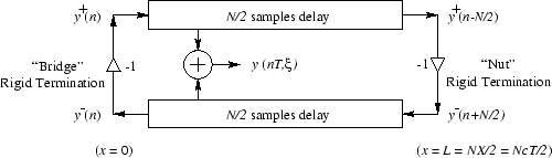
Figure 2: Order N digital waveguide with rigid terminations corresponding to the nut and bridge of a guitar.

The length of the delay lines controls the frequency of oscillation, and consequently the pitch of the output signal. This corresponds to fretting a string on a guitar. Fretting a string limits the vibration to a certain length of the string. This changes the wavelength of the travelling waves, which in turn changes the pitch of the sound. Due to the looping nature of waveguide and the lack of additional input the output at every period is the same except attenuated slightly. Therefore the overall output will be periodic with a period depending to the length of the delay line. Therefore, if the desired frequency of the output is f and the sampling frequency is fs we set each delay line length to N/2 where N = fs/f.

The sound synthesized by this model sounds very artificial. It does nothing to account for the timbre of the instrument, and modeling the string pluck as a triangle wave is not very accurate. In addition, it does not take into account the fact that a real string vibrates in both the horizontal and vertical planes and interacts with the other strings on the guitar. Despite this, it is important to note that it does get a lot right. The damping of the string depends on the frequency - low pitched notes have a lot of sustain whereas high frequency notes attenuate very rapidly. The digital waveguide model simulates this frequency dependant damping effect quite well as can be seen from the sound samples below. It also does a good job creating audible harmonics present in the sound of any stringed instrument. While the basic digital waveguide plucked string model does a good job simulating a generic plucked string, special considerations for the specific instrument being modelled must also be taken into account.

One problem with implementing this system is that the size of the delay lines must be an integer to create a digital filter. If we wish to always use a set sampling frequency, then the delay line lengths will not always be integers. For example to generate the note A4, if our sampling frequency = 44.1 kHz the delay line length would be 44100/370 = 119.189. In this case if we set the delay line length to 119 the output would be of frequency 44100/119 = 370.588. Thus, the resulting output is slightly out of tune. This effect gets greater as the frequency is increased. Another problem with creating this system in the time domain is that it is computationally expensive. Synthesizing a three second tone takes over one minute.

We created a function that works as follows (sampling frequency = 44.1kHz):

y=wav(length,frequency,pick,pickup)
    length = length of output in seconds
    frequency = desired frequency of output
    pick = pick - relative point of pluck [0-1]
    pickup = pickup - relative point of pickup [0-1]

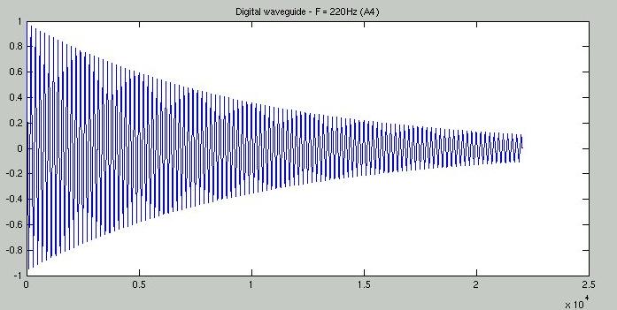
Figure 3: Plot of A4-note generated using the time-domain model. Click here for the wav file. See below for more.

Digital Waveguide Implementation Using Digital Filtering Techniques

To simplify the implementation of the waveguide, the two delay lines can be combined into one, and the damping values at the terminations can be lumped together in the feedback loop (See Figure 4). The -1 multipliers cancel each other out, and the two delay lines can be combined leaving only a length N delay line and the damping factors. The damping factors at each delay can then be lumped together into one damping factor [1].

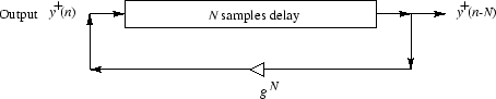
Figure 4: Simplified digital waveguide after combining delay lines and damping factors.

Now the model closely resembles the model originally proposed by Karplus and Strong [2]. However, in a real guitar not all frequencies will decay at equal rates. Therefore, for further realism the lumped damping factor is replaced by a 'loop filter' that damps each frequency differently. This loop filter always has a low pass characteristic to it. In the Karplus-Strong model this loop filter is a single zero FIR filter that averages the Nth and N+1th sample. This corresponds to the following difference equation: Y[k] = .5*(Y[k-N] + Y[k-N-1]).

Another difference in the Karplus-Strong model is that white noise is used as the initial conditions. The periodic nature of the filter creates a steady state output that is of the proper frequency regardless of the initial conditions. Using white noise it is very difficult to accurately reproduce the attack portion of a guitar pluck. In section five we discuss another approach that can more accurately synthesize the attack.

The function we wrote for the Karplus-Strong model works as follows:

function Y=ks(f,length)
   f = desired frequency
   length = length of output in time (seconds)

Figure 5 shows the output of the A4 note generated using the Karplus-Strong model. One can see that this is a great improvement over the results in Figure 3.

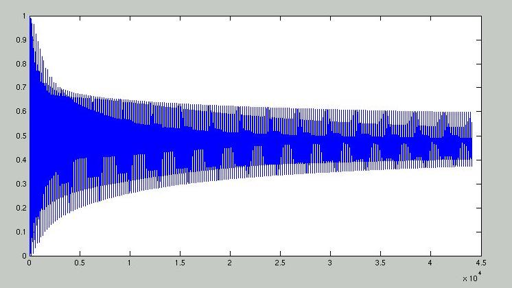
Figure 5: A4 Note genereated using Karplus-Strong model. Click here for the wav file. See below for more.

To simulate the pluck position on the instrument using the simplified model of Figure 4, we can feed the input into an order M comb filter before feeding it into the Karplus-Strong waveguide. The order M is a fraction of N, where N is the length of the delay line, and it determines where the string excitation is applied along the delay line. [1][4]

To fix the fractional delay problem associated with a digital waveguide, it is necessary to interpolate the value at the fractional point along the delay line [4]. Using the example from above for the note A4 we would like to interpolate the value at 'sample' 119.189. We implemented this using a third order Lagrange filter with satisfactory results. This is a linear-phase filter so it doesn't distort the output. Click here for a sample wav file. This is the same note as above A4 though the difference may not be audible.

Loop Filter Design

To accurately model an acoustic guitar, it is necessary to create a loop filter that damps the different harmonics of the fundamental frequency in the same way a real guitar would. This accounts for the effect of the guitar body on the plucked string sound and begins to give the model a timbre similar to that of a real instrument. We followed the procedure presented by Karjalainen, Valimaki and Janosy to create a loop filter based on the recording of a guitar. The algorithm consists of fitting a straight line to the temporal envelopes of a number of early harmonics then using the slopes of the lines to estimate the attenuation factors for those harmonics. Figure 7 shows the temporal envelopes and figure 8 shows the slopes. See [4] for more details.

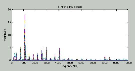
Figure 6: STFT of early harmonics of recorded guitar sound

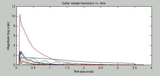
Figure 7: Temporal envelopes of early harmonics.

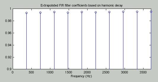
Figure 8: Slopes of time decay of early harmonics.

We had some problems with the design procedure. One problem we had was that initially our desired frequency response was a brickwall filter. This was because we computed the attenuation factors only for the early harmonics and we used zero for the remaining attenuation factors. Therefore our frequency response was essentially an ideal low-pass filter. The result is that our loop filter had a large gain in the transition band. Moreover, an ideal lowpass filter is not even desirable because we want to retain the higher frequencies but they should decay more rapidly than the lower frequencies. Therefore, we computed the attenuation factors of the frequencies above the early harmonics based upon nonzero slopes that decreased linearly as the frequency increased. With a little tweaking we achieved results very similar to those of Karjalainen, V�lim�ki, and J�nosy. However, while they used an iterative approach that weighted the early harmonics more heavily we simply used invfreqz to generate the numerator and denominator of the IIR filter. The resulting filter has the following transfer function:

         0.8995 0.1087z^-1
Hl(z) = -------------------
           1 + 0.0136z^-1

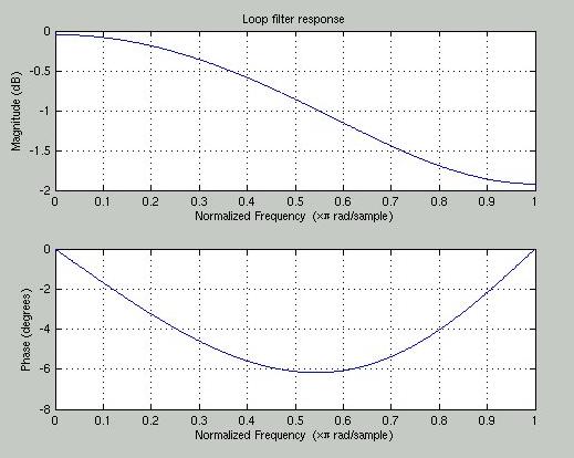
Figure 9: Magnitude and frequency response of the above loop filter. As expected, it has a low pass response so the high frequency harmonics decay faster than the fundamental frequency and the lower frequency harmonics.

The code for this process can be found in loopfilter.m.

Generating Excitation Signals via Inverse Filtering

Once the loop filter has been determined, an excitation signal that is a more accurate model of an actual guitar string pluck can be generated from a recording. This involved putting the recorded signal through the inverse waveguide filter A(z) = 1 - Hl(z)*z^-N where Hl(z) is the loop filter designed above.

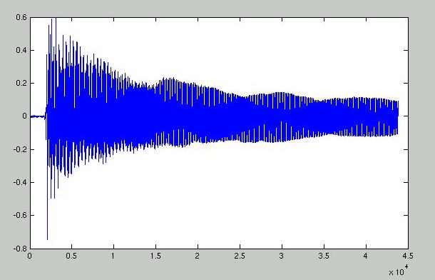
Figure 10: Recording of an F# 4 played by fretting the 7th fret of the B string on an acoustic guitar. wav file

The resulting waveform is a short burst that dies away rather quickly. It consists of a combination of the pluck sound and the impulse response of the guitar body.

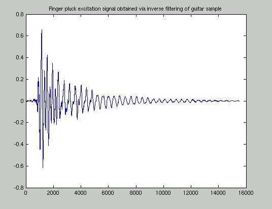
Figure 11: Excitation signal generated by inverse filtering a finger plucked guitar note. wav file. The same excitation signal with the initial string damping removed is also useful. It allows notes to be played in sequence without muting the string between notes. It sounds more realistic under some circumstances (see sound samples below). wav file

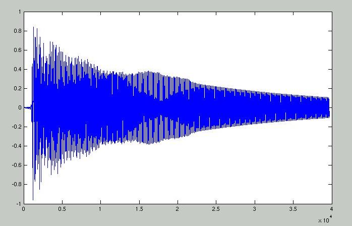
Figure 12: F# 4 (370 Hz) resynthesized using the above excitation signal. wav file

The excitation has a noticeable effect on the attack within the first 500ms (22500 samples). It looks very similar to the attack in the recorded waveform. The difference between the two signals becomes apparent after the attack dies away. The original signal attenuates more rapidly and is missing the very low frequency components of the original sound. Despite this, it sounds almost identical to the original note.

Overall, using the excitation signals generated using this technique offers a large improvement in sound quality over white noise or some other artificial excitation signal as it is based on the actual excitation that is applied to a guitar string. It takes into account the effect that the guitar body has on the string excitation, resulting in an even more accurate model. This process can be used to simulate different plucking techniques as well, resulting in a an even more versatile model. We have generated excitation signals based on a finger picked string with different attacks, and using a pick. See below for wav files of different excitation signals, as well as more sound samples. Overall the best results were obtained using finger plucked excitation signals. The pick signals sound very harsh when compared to the others.

The code to generate these excitation signals can be found in getexcitesignal.m. It can be used as follows:

y=getexcitesignal(B, A, W, f, fs)
 B = numerator coeeficients of loop filter 
 A = denominator coeeficients of loop filter 
 W = sound sample to filter
 f = fundamental frequency of W
 fs = sampling frequency

Bringing it all together

Below is the block diagram of the final filter we have designed to synthesize an acoustic guitar:

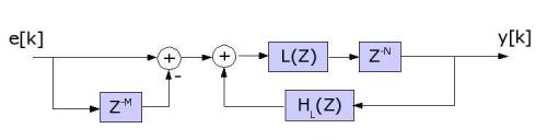
Figure 13: Block diagram of the final filter.

One can see the length N delay line from the original Karplus-Strong digital waveguide model. The Lagrange interpolation filter (L(Z)) feeds into the delay line for proper tuning. It also has an improved loop filter (H_L(Z)) based on recordings from an actual guitar. A comb filter has been placed at the input (the left-hand portion of the block diagram) to simulate the effect of plucking position on guitar. The input to the system is an excitation signal (e[k]) obtained through inverse filtering of a guitar recording. The results are quite convincing. See Synthesized Sounds for some samples.

The code for this filter can be found in kspluck.m. It can be used as follows:

    kspluck(f, length, fs, excitation, B, A, p) 
    f = frequency
    length = duration of note (seconds)
    fs = sampling freqency
    excitation = string excitation signal
    B = numerator coefficients of loop filter
    A = denominator coefficients of loop filter
    p = pluck position along waveguide (0 < p<  1 - fraction of waveguide length)

Conclusions and Future Work

We have observed one important problem with our model. As one can tell from some of the sound samples below, there is a high frequency ringing in some of the notes synthesized using the pick excitation signal that we were unable to remove. In addition when using kspluck.m to synthesize A notes (at any octave) with the excitation signals we generated, the magnitude of the output is approximately twice that of other notes, which causes it to clip when saved to a wav file. This is because there is a large frequency component of the excitation signal at 220Hz, which leads to this resonance. The solution to these problems is creating more excitation signals based on other guitar notes. If we were to generate more excitation signals from various positions on the guitar's fretboard and only use excitations based on notes located only a few frets away we would be able to get a far more accurate model. This may sound like a large disadvantage, but it would still take relatively few excitation signals to accurately model all the notes that can be played on a guitar. Despite these drawbacks, we feel that even with a few improvements to the basic plucked string model we were able to synthesize very realistic sounds. Estimating the model parameters based on a real instrument had the largest effect on the resulting quality, resulting in a very guitar-like timbre. While consideration must be given to other factors, we believe that they will contribute less overall to the accuracy of the synthesized sound.

References

1. Smith, Julius O. Digital Waveguide Modeling of Musical Instruments, Center for Computer Research in Music and Acoustics (CCRMA), Stanford University, 2003-12-10. Web published at http://www-ccrma.stanford.edu/~jos/waveguide/
2. K.�Karplus and A.�Strong, ``Digital synthesis of plucked string and drum timbres,'' Computer Music Journal, vol.�7, no.�2, pp. 43-55, 1983, Reprinted in [4].
3. D.A. Jaffe and J.O. Smith, ``Extensions of the Karplus-Strong plucked string algorithm,'' Computer Music Journal, vol.�7, no.�2, pp. 56-69, 1983, Reprinted in [4].
4. C.Roads, ed., The Music Machine,
   Cambridge, MA: MIT Press, 1989.
5. M. Karjalainen, V. V�lim�ki, and Z. J�nosy, ``Towards high-quality sound synthesis of the guitar and string instruments,'' in Proceedings of the 1993 International Computer Music Conference, Tokyo, pp. 56-63, Computer Music Association, Sept. 10-15 1993, available online at http://www.acoustics.hut.fi/~vpv/publications/icmc93-guitar.htm.
6. Dan Ellis - plucked string model available online at http://www.ee.columbia.edu/~dpwe/resources/matlab/pluck.html

Code index

1. notes.m- defines some arrays of notes and their associated frequencies.
2. wav.m - Simple digital waveguide plucked string model.
3. ks.m - Karplus-Strong plucked string model.
4. ksintune.m - Karplus-Strong plucked string model with Lagrange interpolation fractional delay filter.
5. lagrange.m - code to generate an FIR Lagrange interpolation filter
6. loopfilter.m - analizes guitar recording to estimate the corresponding loop filter based on the decay rate of the harmonics.
7. getexcitesignal.m - puts input recorded signal through an inverse digital waveguide filter to extract the excitation signal.
8. ksloop.m - Karplus-Strong plucked string model - takes the loop filter coefficients and excitation signal as arguments.
9. kspluck.m - Our final guitar model - includes all of the above modifications (fractional delay compensation, loop filter input, excitation signal input) as well as a comb filter at the input to model different pluck positions along the string.
10. mary.m - plays Mary Had a Little Lamb using kspluck.m
11. ksmary.m - plays Mary Had a Little Lamb using ks.m
12. wavmary.m - plays Mary Had a Little Lamb using wav.m

Sound index

1. Recordings

   1. Bstring 7thfret-picked.wav - recording of a guitar fretted at the 7th fret on the B string (F# 4 = 370 Hz) using a pick.
   2. Bstring 7thfret-plucked.wav - recording of a guitar fretted at the 7th fret on the B string (F# 4 = 370 Hz) finger plucked.

2. Excitation signals

   1. excite-plucked.wav - finger plucked string excitation signal with harsh attack
   2. excite-plucked-soft.wav - finger plucked string excitation signal with softer attack
   3. excite-plucked-nodamp.wav - finger plucked string excitation signal without initial damping
   4. excite-picked.wav - picked string excitation signal
   5. excite-picked-nodamp.wav - finger plucked string excitation signal without initial damping

3. Synthesized sounds

   1. waveguide-A4.wav - Synthesized A 4 (220 Hz) using the basic digital waveguide plucked string model
   2. waveguide-B3.wav - Synthesized B 3 (123.48 Hz) using the basic digital waveguide plucked string model
   3. wavmary.wav - Mary Had a Little Lamb played with wav.m (it takes a long time to run).
   4. ks-A4.wav - A 4 synthesized using Karplus-Strong plucked string model
   5. ks-B3.wav - B 3 synthesized using Karplus-Strong plucked string model
   6. ksmary.wav - Mary Had a Little Lamb played using ks.m
   7. ks-lagrange-A4.wav - A 4 synthesized using Karplus-Strong plucked string model with Lagrange interpolation filter - this one is actually in tune.
   8. kspluck-B3.wav - B3 using kspluck.m with loop filter created by loopfilter.m
   9. kspluck-F4.wav - higher pitch note (F4) using kspluck.m with loop filter created by loopfilter.m
   10. mary-plucked.wav - Mary Had a Little Lamb using finger plucked excitation signal with a somewhat harsh attack. Based on our final guitar model.
   11. mary-plucked-soft.wav - Mary Had a Little Lamb using finger plucked excitation signal with a softer attack. Based on our final guitar model.
   12. mary-picked.wav - Mary Had a Little Lamb using picked excitation signal. Based on our final guitar model.
   13. mary-plucked-nodamp.wav - Mary Had a Little Lamb using finger plucked excitation signal, without muting the strings between each note. Based on our final guitar model.
   14. mary-picked-nodamp.wav - Mary Had a Little Lamb using picked excitation signal, without muting the strings between each note. Based on our final guitar model.
   15. mary-4thoctave.wav - Mary Had a Little Lamb using plucked-soft excitation signal played an octave higher. Based on our final guitar model.