Lecture 1: Matlab DSP Review

Contents

Simple signals

Generate a pure tone.

% Pick a sampling rate.
sr = 8000;
% Define the time axis.
dur = 1; % sec
t = linspace(0, dur, dur * sr);
freq = 440; % Hz
x = sin(2*pi*freq*t);

Playing sounds.

soundsc(x, sr)

Warning: The playback thread did not start within one second.
(Type "warning off MATLAB:audioplayer:playthread" to suppress this warning.) 

Making plots.

plot(t, x)
xlabel('Time (sec)')

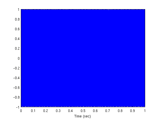
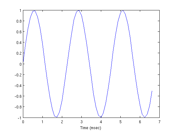
That looks pretty terrible. Lets only plot the first few cycles.

period = 1.0 / freq; % sec
samples_per_period = period * sr;
idx = 1:3*samples_per_period;
plot(t(idx) * 1e3, x(idx));
xlabel('Time (msec)')

Make some noise.

% rand generates uniformly distributed random values between 0 and 1.
n = rand(1, length(t)) - 0.5;
plot(t(idx) * 1e3, n(idx))
xlabel('Time (msec)')

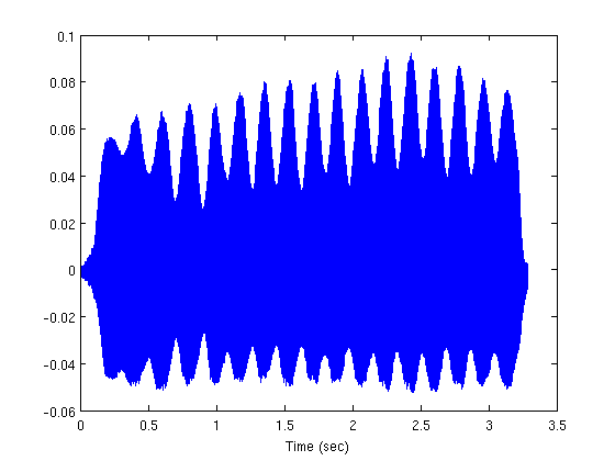
Audio I/O

filename = 'flute-C4.wav';
[x2 sr2] = wavread(filename);

% Get the time axis right.
t2 = linspace(0, length(x2) / sr2, length(x2));
plot(t2, x2)
xlabel('Time (sec)')

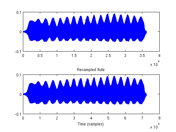
Resampling

sr3 = 4000; % Hz
x3 = resample(x2, 8000, sr3);
subplot(211)
title('Flute')
plot(x2)
subplot(212)
plot(x3)
title('Resampled flute')
xlabel('Time (samples)')

Write the sound file to disk.

wavwrite(x3, sr3, 'flute-resampled.wav')

Fourier Transform

X = fft(x);

Whats the frequency axis?

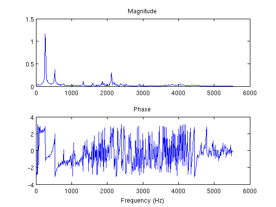
f = linspace(0, sr, length(X));
subplot(211)
plot(f, abs(X))
title('Magnitude')
subplot(212)
plot(f, angle(X))
title('Phase')
xlabel('Frequency (Hz)')

Recall that for real-valued signals the DFT is always symmetric around sr/2 (or 0), so we only need to plot the first half. This time for x2.

X2 = fft(x2(1:1024));
f2 = linspace(0, sr2, length(X2));
subplot(211)
plot(f2(1:end/2+1), abs(X2(1:end/2+1)))
title('Magnitude')
subplot(212)
plot(f2(1:end/2+1), angle(X2(1:end/2+1)))
title('Phase')
xlabel('Frequency (Hz)')

Whats the (approximate) fundamental frequency of the flute note (C4)? Just find the bin corresponding to the first peak in the magnitude spectrum.

mag = abs(X2);
% Ignore redundant second half.
mag = mag(1:end/2+1);
% Find all local maxima.
peaks = (mag(1:end-2) < mag(2:end-1)) & mag(2:end-1) > mag(3:end);
length(peaks)

ans =
   511

But we only want the peaks above a threshold to ensure that we ignore the noise.

peaks = peaks & mag(2:end-1) > 0.5;
f2(peaks)

ans =
       247.87

Filters

Simple FIR filter: y[n] = 0.5*x[n] + 0.5*x[n-1]

filt = [0.5, 0.5];

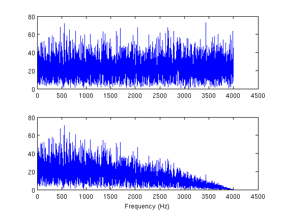
Lets filter some noise buy convolving it with the impulse response.

% Recall that the convolution of two signals with length N1 and N2 is
% N1 + N2 - 1.  The 'same' argument just tells conv to truncate the
% convolved signal at N1 samples.
y = conv(n, filt, 'same');
N = fft(n);
Y = fft(y);
idx = 1:length(n) / 2 + 1;
subplot(211); plot(f(idx), abs(N(idx)))
subplot(212); plot(f(idx), abs(Y(idx)))
xlabel('Frequency (Hz)')

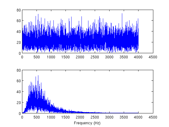
What about IIR filters?

[b a] = butter(2, [400 1500]/sr)
y = filter(b, a, n);
Y = fft(y);
subplot(212); plot(f(idx), abs(Y(idx)))
xlabel('Frequency (Hz)')

b =
     0.035438            0    -0.070875            0     0.035438
a =
            1      -3.2428       4.0778      -2.3717      0.54317

(You can use filter for FIR filters too, just be sure that the second argument is a scalar).

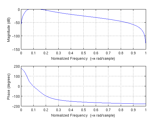
Matlab has a special function to plot a filter's frequency response.

clf
freqz(b, a)

Pole-zero plots too:

zplane(b, a)

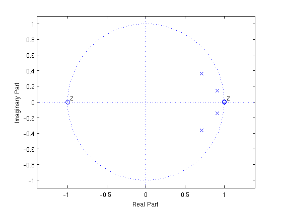
Lets make an unstable filter.

b = 1;
a = [1 2];
zplane(b, a)

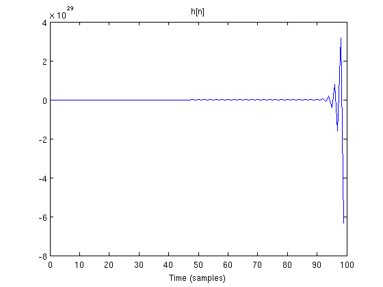
That pole is definitely outside of the unit circle. What is its impulse response?

[h, t] = impz(b, a, 100);  % Get first 100 samples of impulse response
plot(t, h)
title('h[n]')
xlabel('Time (samples)')

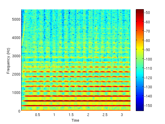
Spectrograms

nwin = 512; % samples
noverlap = 256; %samples
nfft = 512; %samples
spectrogram(x2, nwin, noverlap, nfft, sr2, 'yaxis');
colorbar

Getting help

lookfor spectrogram

specgram                       - Spectrogram using a Short-Time Fourier Transform (STFT).
spectrogram                    - Spectrogram using a Short-Time Fourier Transform (STFT).
specgramdemo                   - Spectrogram Display.

help spectrogram

 SPECTROGRAM Spectrogram using a Short-Time Fourier Transform (STFT).
    S = SPECTROGRAM(X) returns the spectrogram of the signal specified by
    vector X in the matrix S. By default, X is divided into eight segments
    with 50% overlap, each segment is windowed with a Hamming window. The
    number of frequency points used to calculate the discrete Fourier
    transforms is equal to the maximum of 256 or the next power of two
    greater than the length of each segment of X.
 
    If X cannot be divided exactly into eight segments, X will be truncated
    accordingly.
 
    S = SPECTROGRAM(X,WINDOW) when WINDOW is a vector, divides X into
    segments of length equal to the length of WINDOW, and then windows each
    segment with the vector specified in WINDOW.  If WINDOW is an integer,
    X is divided into segments of length equal to that integer value, and a
    Hamming window of equal length is used.  If WINDOW is not specified, the
    default is used.
 
    S = SPECTROGRAM(X,WINDOW,NOVERLAP) NOVERLAP is the number of samples
    each segment of X overlaps. NOVERLAP must be an integer smaller than
    WINDOW if WINDOW is an integer.  NOVERLAP must be an integer smaller
    than the length of WINDOW if WINDOW is a vector.  If NOVERLAP is not
    specified, the default value is used to obtain a 50% overlap.
 
    S = SPECTROGRAM(X,WINDOW,NOVERLAP,NFFT) specifies the number of
    frequency points used to calculate the discrete Fourier transforms.
    If NFFT is not specified, the default NFFT is used. 
 
    S = SPECTROGRAM(X,WINDOW,NOVERLAP,NFFT,Fs) Fs is the sampling frequency
    specified in Hz. If Fs is specified as empty, it defaults to 1 Hz. If 
    it is not specified, normalized frequency is used.
 
    Each column of S contains an estimate of the short-term, time-localized
    frequency content of the signal X.  Time increases across the columns
    of S, from left to right.  Frequency increases down the rows, starting
    at 0.  If X is a length NX complex signal, S is a complex matrix with
    NFFT rows and k = fix((NX-NOVERLAP)/(length(WINDOW)-NOVERLAP)) columns.
    For real X, S has (NFFT/2+1) rows if NFFT is even, and (NFFT+1)/2 rows
    if NFFT is odd.  
 
    [S,F,T] = SPECTROGRAM(...) returns a vector of frequencies F and a
    vector of times T at which the spectrogram is computed. F has length
    equal to the number of rows of S. T has length k (defined above) and
    its value corresponds to the center of each segment.
 
    [S,F,T] = SPECTROGRAM(X,WINDOW,NOVERLAP,F,Fs) where F is a vector of 
    frequencies in Hz (with 2 or more elements) computes the spectrogram at 
    those frequencies using the Goertzel algorithm. The specified 
    frequencies in F are rounded to the nearest DFT bin commensurate with 
    the signal's resolution. 
 
    [S,F,T,P] = SPECTROGRAM(...) P is a matrix representing the Power
    Spectral Density (PSD) of each segment. For real signals, SPECTROGRAM
    returns the one-sided modified periodogram estimate of the PSD of each
    segment; for complex signals and in the case when a vector of
    frequencies is specified, it returns the two-sided PSD.  
 
    SPECTROGRAM(...) with no output arguments plots the PSD estimate for
    each segment on a surface in the current figure. It uses
    SURF(f,t,10*log10(abs(P)) where P is the fourth output argument. A
    trailing input string, FREQLOCATION, controls where MATLAB displays the
    frequency axis. This string can be either 'xaxis' or 'yaxis'.  Setting
    this FREQLOCATION to 'yaxis' displays frequency on the y-axis and time
    on the x-axis.  The default is 'xaxis' which displays the frequency on
    the x-axis. If FREQLOCATION is specified when output arguments are
    requested, it is ignored.
 
    EXAMPLE 1: Display the PSD of each segment of a quadratic chirp.
      t=0:0.001:2;                    % 2 secs @ 1kHz sample rate
      y=chirp(t,100,1,200,'q');       % Start @ 100Hz, cross 200Hz at t=1sec 
      spectrogram(y,128,120,128,1E3); % Display the spectrogram
      title('Quadratic Chirp: start at 100Hz and cross 200Hz at t=1sec');
 
    EXAMPLE 2: Display the PSD of each segment of a linear chirp.
      t=0:0.001:2;                    % 2 secs @ 1kHz sample rate
      x=chirp(t,0,1,150);             % Start @ DC, cross 150Hz at t=1sec 
      F = 0:.1:100;
      [y,f,t,p] = spectrogram(x,256,250,F,1E3,'yaxis'); 
      % NOTE: This is the same as calling SPECTROGRAM with no outputs.
      surf(t,f,10*log10(abs(p)),'EdgeColor','none');   
      axis xy; axis tight; colormap(jet); view(0,90);
      xlabel('Time');
      ylabel('Frequency (Hz)');
 
    See also PERIODOGRAM, PWELCH, SPECTRUM, GOERTZEL.

    Reference page in Help browser
       doc spectrogram

Graphical documentation

doc spectrogram

Advanced Matlab audio processing resources: http://www.ee.columbia.edu/~dpwe/resources/matlab/

author = 'Ron Weiss <[email protected]>';
fprintf('%s\nLast updated %s\n', author, datestr(now))

Ron Weiss <[email protected]>
Last updated 21-Jan-2010 17:30:18

Published with MATLAB® 7.8