Manuel Reyes-Gomez
Nebojsa Jojic
Daniel P.W. Ellis
Columbia University
Microsoft Research Columbia University
! WATCH THE TEN VIDEOS BELOW !
I.- INTRODUCTION
In many audio signals including speech and musical instruments,
there is high correlation
between adjacent frames of their spectral representation.
Our approach consists in exploiting
this correlation so that explicit models are required
for those frames that cannot be accurately
predicted from their context.
Our model captures the general properties of such audio
sources by modeling the evolution
of their harmonics components. Using the common source-filter
model for such signals, we
devise a layered generative model that describes these
two components in separate layers:
one for the excitation harmonics, and another for resonances
such as vocal tract formants.
Our approach explicity models the self-similarity and
dynamics of each layer by fitting the
log-spectra in frame t with a set of transformations
of the log-spectra in frame t-1. As a result,
we do not require separate states for every possible
spectral configuration,but only a limiter
set of "sharp" states that can still cover the full spectral
veriety of a source via such
transformations. This approach is thus suitable for any
time series data with high correlation
between adajacent observations.
We will first introduce a model that captures the spectral
deformation field of the speech
harmonics, and show how this can be explioted to interpolate
mising observations. Then, we
introduce the two-layer model that separately models
the deformation fields for harmonic
and formant resonance components, and show that such
a separation is necessary to
accurately describe speech signals through examples of
the missing data scenario with
one and two layers
Then we will present the complete model including the
two deformation fields and the
"sharp" states This model, with only a few states
and both deformation fields, can
accurately reconstruct the signal.
Finally, we briefly describe a rang of exisitng applications
including semi-supervised source
separation, and discuss the model's possible application
to unsupervised source separation.
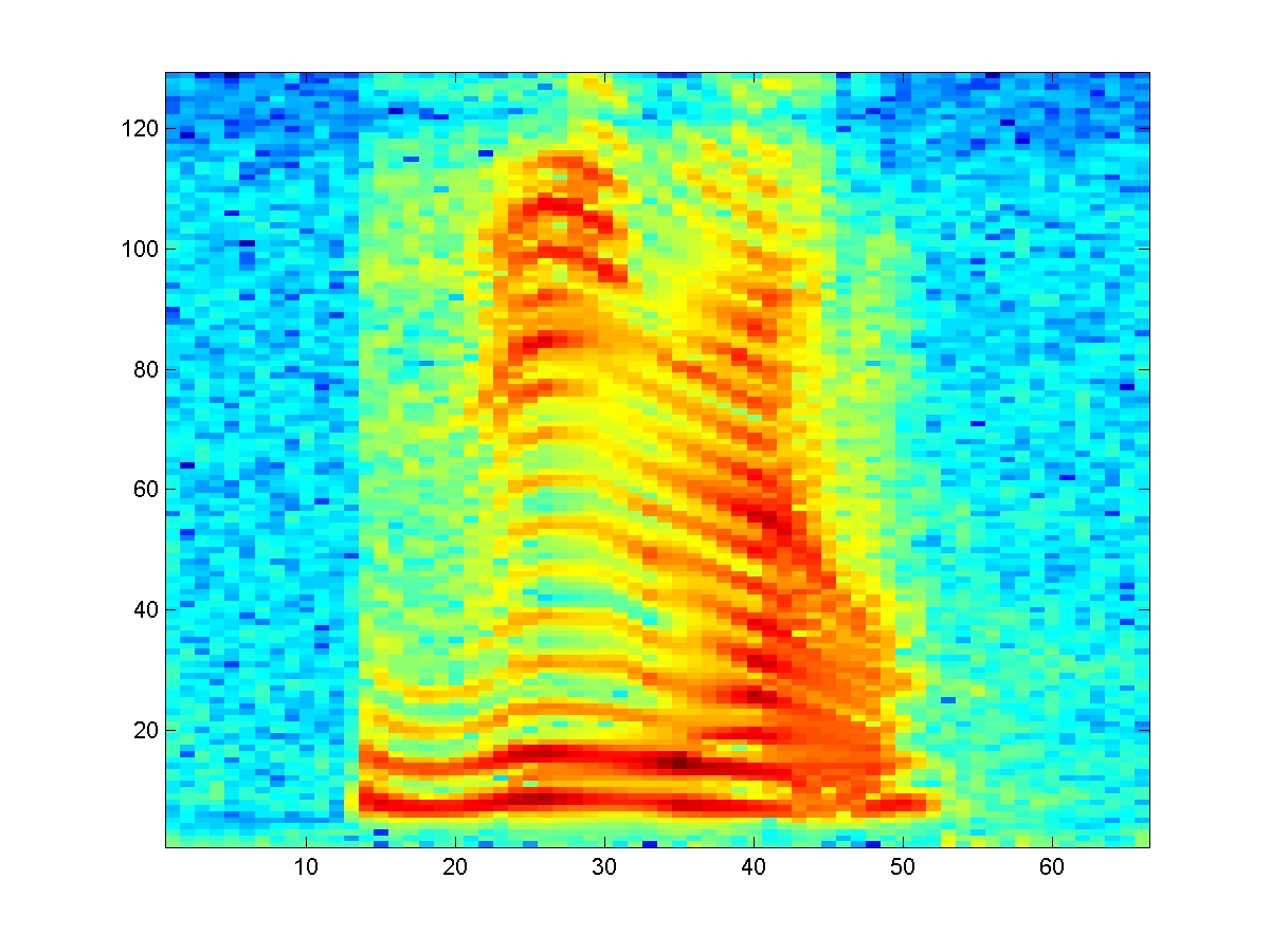
II.- SPECTRAL DEFORMATION MODEL
Figure 1 shows a narrow band spectrogram representation
of a speech signal, where each
column depicts the energy content across frequency in
a short-time window, or time-frame.
The value in each cell is actually the log-magnitude
of the short-time Fourier transform.
![]()
Figure 1
Using the subscript C to designate current and P to indicate
previous, the model predicts
a patch of Nc time-frequency bins centered at the kth
frequency bin of frame t as a
``transformation'' of a patch of Np bins around
the kth bin of frame t-1.
Figure 1, shows an example with Nc = 3 and Np = 5 to illustrate
the intuition behind this
approach. The selected patch in frame t can be seen as
a close replica of an upward shift
of part of the patch highlighted in frame t-1.
This ``upward'' relationship can be captured by a
transformation matrix such as the one shown in the figure.
The patch in frame t-1 is larger than the patch in frame
t to permit both upward and
downward motions.
The generative graphical model for a single layer is depicted in figure 2.
![]()
Figure 2: a)Graphical model; b) Graphical simplification
X nodes correspond to the observations, and T nodes to
the tranformations at each frequency
bin. At each bin, the local likelihood potentials involve:
the Nc bins used in the current frame,
the Np bins used in the previous frame and the set of
all possible transformation matrix defined
by T. Please read the paper for complete details.
Inference is efficiently performed via loopy belief propagations.
Once the posteriors of the
transformation nodes are estimated, we can find
the "expected" transformation maps an
appealing description of the harmonic's dynamics, as
can be observed in figure 3.
In these panels, the links between three specific time-frequency
bins and their corresponding
transformations on the map are highlighted. Bin 1 is
described by a steep downward
transformation, while bin 3 also has a downward motion
but is described by a less steep
transformation, consistent with the dynamics visible
in the spectrogram. Bin 2, in other hand,
is described by a steep upwards transformation.
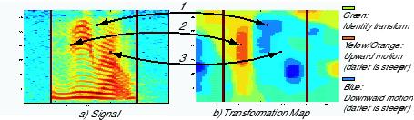
Figure 3.- Tranformation Map. Green : Identity transform;
Yellow/Orange : Upward Motion, darker is steeper.
Blue : Downward motion; darker is steeper.
DEMO INTRODUCTION
We have built a real time demo that performs a variety of applications using this model.
The user can change the different parameters of the model
on the user interfase, (Figure 4).
There are several panels and function buttons that we
will explain using different applications.
The information displayed on each panel changes with
each application.
We will present ten short videos of the demo for
each application. Before each video we
will describe the application, the information displayed
in each panel and the functionality of
the buttons.
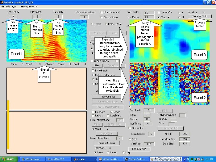
Description of Video 1.
We first present an instance on the demo performing basic
estimation of the harmonics
transformation maps followed by a harmonics tracking
application.
Figure 4, shows a typical "screen shot" of the demo for
this application. The figure displays
three panels. Panel 1: displays the signal to be processed;
Panel 2: Shows the most likely
tranformation obtained from the local likelihood potential,
here as in the transformations maps,
the color relates to the motion present in the signal,
however the structure is not clearly
defined as in the transformations maps, also notice
the total lack of a clear structure on the
silent regions of the signal.; Panel 3: Shows the transformation
maps obtained after each
complete iteration.
Each complete iteration consists on complete belief propagation
messages passes through all
the vertical chains, each vertical chain consist in all
the coefficients for a given frame, followed
by the complete belief propagation passes on all the
horizontal chains, each horizontal frame
consist in all the frames for a given coefficient, the
belief propagation rules for this chains can be
implemented using efficient forward/backward, upward/downward
recurssions, see extended
paper for details. The strength of the belief propagation
in each direction is controlled by transition
potentials in each direction. Parameters "Ver. Factor"
and "Hor. Factor" affect the probability of
switching to a different transform, a higher value on
this factor results in "smother" transformation
patterns on that direction. The video also shows the
effect of changes on those
factors.
Once the transformation maps are estimated, some interesting
applications can be performed,
like tracking harmonics. The user "clicks" in a certain
region of the spectrogram, and if the
"Track H" button is pushed, the demo shows the history
of that particular time-frequency bin.
VIDEO 1. - Harmonics transformations
maps and harmonics
tracking application.
CLICK ON THE SCREEN TO ACTIVE THE VIDEO !
III.- MISSING DATA SCENARIO
If parts of the spectrogram are corrupted or missing like
in figure 5 a), we can "fill in" those values
by considering the correspondent parts of variables X
as hidden, and propagating continuous
"belief" messages from and to the hidden nodes, we use
again belief propagation. The posteriors
of the continuous hidden nodes is approximated using
a gaussian distributions. The missing values
are then "filled in" with the means of their posterior
distributions. Check the full sequence of
iterations on Video 2.
CLICK ON SIGNALS TO HEAR THE RECONSTRUCTED SPEECH !


Figure 5
a) Original Occluded Signal
b) Filled in signal after 5 iterations
c) Filled in signal after 10 iterations


d) Filled in signal after 20 iterations
e) Filled in signal after 30 iterations
f) Filled in signal after 40 iterations
Description of Video 2.
The video presents the missing data application using
a single layer model. This time four panels are
used. Panel 1 is first used to defined the missing
regions, once the "Fill In" button is pressed the
missing regions are estimated with the "filled in" values.
Panel 2, as before shows the local
likelihood potentials, when the observation of a particular
time-frequency bin is missed, no reliable
local likelihood potential can be estimated, and therefore
any local "belief" regarding the identity
of the correct transformation can be transmited to the
correspondent transformation node. Then,
we set the correspondent messages from the local likelihood
potentials to the transformation nodes
as uniform. The transformation posteriors (Panel 3) are
estimated as before using the "new" local
likelihood potentials, therefore the transformation posteriors
on the "missing" regions are driven
entirely by the tranformation "beliefs" of their reliable
neighbors. We keep the transformation
posteriors fixed and then we start propagating the continuous
messages and the missing values begin
to be filled, once we have some "meaningful" information
on the missing regions we start to
calculate the local potentials on the missing regions
using the "filled in" values and the
transformation posteriors are frequently reestimated.
Panel 4, show the original signal for
comparison purposes only.
VIDEO 2.- Missing Data Application.
CLICK ON THE SCREEN TO ACTIVE THE
VIDEO !

Description of Video 3.
This is one is similar to the previous one, it also shows
the "fill in" application with a single
layer. The purpose of this video is to illustrate that
belief propagation is not "magic", and
that when a single missing region is too big, the reliable
neighbors are to apart to propagate
the right transformations "beliefs" to their missing
neighbors. However the perceptual
results obtained are significantly better than the signal
with "missing regions".
VIDEO 3.- Missing Data Application. Severe Case
CLICK ON THE SCREEN TO ACTIVE THE VIDEO !

IV.- TWO LAYER SOURCE-FILTER TRANFORMATIONS
Many sound sources, including voiced speech, can be successfully
regarded as the convolution of a
broad-band source excitation, such as the pseudo-periodic
glottal flow, and a time-varying
resonant filter, such as the vocal tract,
that `colors' the excitation to produce speech sounds or
other distinctions.
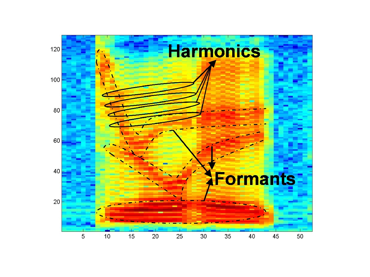
When the excitation has a spectrum consisting of well-defined
harmonics, the overall spectrum is
in essence the resonant frequency response sampled at
the frequencies of the harmonics.
Figure 6, shows an spectrogram where the harmonics and the formants are clearly shown.
Since convolution of the source with the filter in the
time domain corresponds to multiplying
their spectra in the Fourier domain, or adding in the
log-spectral domain. Hence, we model
the log-spectra X as the sum of variables F and H, which
explicitly model the formants and
the harmonics of the speech signal. The source-filter
transformation model is based on two
additive layers of the deformation model described above,
as illustrated in figure 7.

Figure 7
Variables F and H in the model are hidden, while, as before,
X can be observed or hidden.
The symmetry between the two layers is broken by using
different parameters in each,
chosen to suit the particular dynamics of each component.
We use transformations with a larger support in the formant
layer compared to the
harmonics layer. Since all harmonics tend to move in
the same direction, we enforce smoother
transformation maps on the harmonics layer by using potential
transition matrices with a higher
self-loop probabilities.
Figure 8, shows the decomposition of a speech signal into
harmonics and formants
components, illustrated as the means of the posteriors
of the continuous hidden variables
in each layer.

Figure 8
The decomposition is not perfect; Since we separate the
components in terms of differences
in dynamics, this criteria becomes insufficient when
both layers have similar motion.
Separation improves modeling precisely when each component
has a different motion, and
when the motions coincide is not really important in
which layer the source is actually captured.
However, some applications may require a better separation,
which is part of our current
research.
Figure 9; b) shows the spectrogram of part a) with a "mising"
region; notice that the two
layers have distinctly different motions. In c)
the region has been filled via inference
in a single-layer model; Notice that since the
formant motion does not follow the harmonics,
the formants are not captured in the reconstruction.
In d) the two layers are first decomposed
and then each layer is filled in; the figure shows the
addition of the filled-in version in each layer.
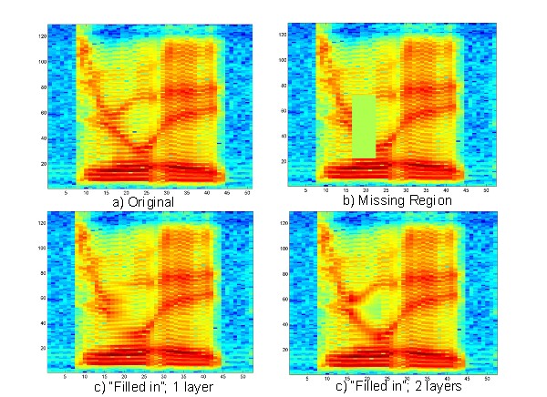
Figure 9
Description of Video 4.
This video illustrates the need of a model that takes
in account the production model for
voiced speech, the video shows a single layer "fill in"
application, where the "missing"
harmonics are correctly regenerated while falling to
regenerate some of the "missing"
formants. The panels display the same information as
in the previous two videos.
VIDEO 4.- One layer; Missing
Data Application;
Introducing the need for two
layers.
CLICK ON THE SCREEN TO ACTIVE THE VIDEO !

Description of Video 5.
This video performs harmonics/formants separation. The
screen has 5 panels. Panel 1, shows
the original spectrogram; Panels 2: Displays the
estimated means for the harmonics posteriors
Panels 3: Displays the estimated means for the formants
posteriors; Panel 4: Displays the
transformation maps for the harmonics layer; Panel 5:
Displays the transformation maps for the
formants layer.
VIDEO 5.- Harmonics/Formants Separation.
CLICK ON THE SCREEN TO ACTIVE THE
VIDEO !

Description of Video 6.
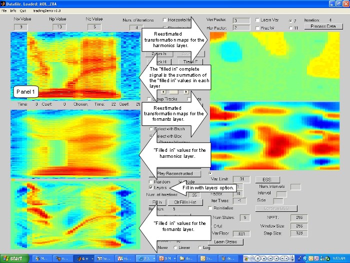
This video performs the two layers missing data application.
Here each layer is "filled in"
independently, as before the transformation maps for
each layer are reestimated using uniform
messages from the local likelihood potentials on the
"missing" regions. The complete spectrogram
is "filled in" with the summation of the "filled in"
versions on each layer.
The screen has 5 panels. Panel 1, shows the complete
spectrogram with the "filled in" values;
Panels 2: Displays the "filled in" values for the harmonics
layers; Panels 3: Displays the "filled in"
values for the formants layer; Panel 4: Displays
the transformation maps for the harmonics layer;
Panel 5: Displays the transformation maps for the formants
layer.
VIDEO 6.- Two layers Missing Data Application.
CLICK ON THE SCREEN TO ACTIVE THE VIDEO !
V.- Matching-Tracking Model
Prediction of frames from their context is not always
possible such as when there are transitions
between silence and speech or transitions between voiced
and unvoiced speech, so we need a
set of states to represent these unpredictable
frames explicitly.
We will also need a second ``switch'' variable that will
decide when to ``track'' (transform) and
when to ``match'' the observation with a state.
Figure 10, shows a graphical representation of this
model. At each time frame, discrete variables St
and Ct are connected to all frequency bins in that
frame. St is a uniformly-weighted GMM containing
the means and the variances of the states to
model. Variable Ct takes two values: When
it is equal to 0, the model is in ``tracking mode''; a value
of 1 designates ``matching mode''.
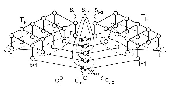
Figure 10
The potentials between variables St ,
Ct , Xt, Ft and Ht are described
in the paper.
The posteriors for variables St
and Ct (Q(St ) and Q(Ct )) are obtained
using the
belief propagation rules, Q(Ct = 0) is large
if the match between the current frame
and its prediction from the context it larger than the
match between the current
frame and the means set of the GMM. In early iterations
when the means are still
quite random, the match between the means set and
the observations is pretty low,
making Q(Ct = 0) large with the result
that the explicit states are never used.
To prevent this we start the model with large variances,
which will result in
non-zero values for Q(Ct=1), and hence the
explicit states will be learned.
As we progress, we start to learn the variances. When
the variances are large, most
of the frames are used in learning the means sets, typically
resulting in a set of similar
"blurry" states, however as the variances start to be
learned and become smaller
Q(Ct=1) takes non-zero values only in very
few frames, selecting those few frames to
learn the means set, resulting in "sharper" means.
We start with a relative large number of means, but this
becomes much smaller once
the variances are learned; The resulting states typically
consist of single frames at
discontinuities as intended. Figure 11 a) shows the frames
chosen for the spectrogram
on figure 1. The signal reconstruction is done
by using the correspondent chosen frames
on the two layers. The reconstruction is simply
another instance of inferring missing
values, except the motion fields are not reestimated
since we have the true ones.
Figure 11 shows several stages of the reconstruction.
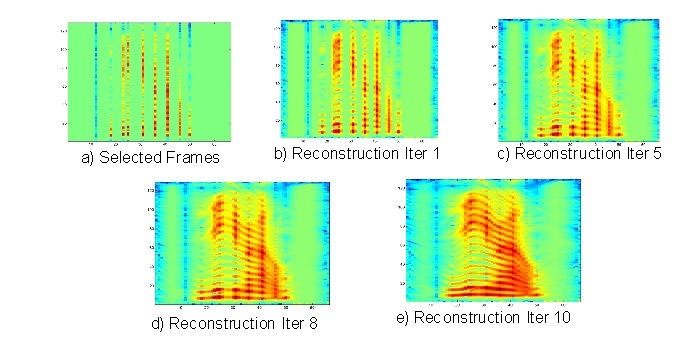
Figure 11
Videos 7 and 10 provide a good insigth of how this model operates.
Description of Video 7.
In this video, the matching-tracking model is applied
on a single source signal. The video is
divided in two parts. The estimation of the model and
the reconstruction of the signal spectrogram
from the model parameters. As we mentioned above
some care with the model variances has to be
taken to ensure the adequate estimation of the model
parameters. We keep the variances large for
the early stages of the model estimation, while learning
them in the later stages. We present and
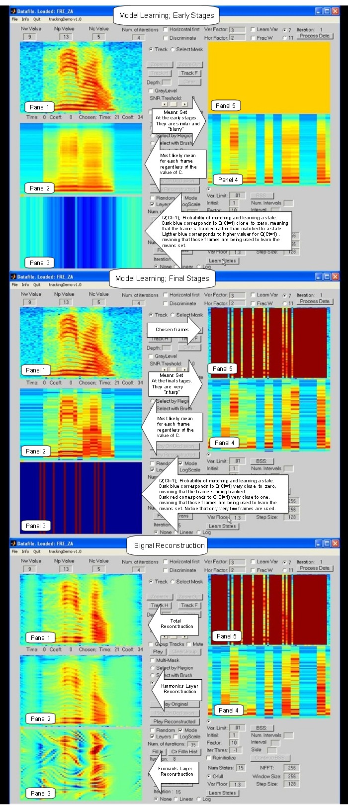
briefly discuss three screen shots for this video.
During model estimation, the demo displays information
in 4 panels. Panel 1, displays the signal to
be modeled. Panel 4 displays the means set for the states
of variable St; Panel 2 displays the mean
of the most likely state for each frame; Panel 3 shows
the values of the posteriors for Ct = 1;
i.e. the probability that the model matchs frame t with
a state from variable St, rather than tracking,
(estimating) the frame from its context.
In panel 3, frames in dark blue correspond to those frames
where Q(Ct=1) is close to zero, meaning
that the frame is tracked rather than matched to a state,
frames in dark red correspond to those frames
where Q(Ct=1) is close to one, meaning that
the frame is used to learn the states during the model
estimation. Frames with colors in between are partially
tracked and partially matched to a state and they
are also partially used to learn the states during the
model estimation, notice that this is the case during
the early stages of the model estimation procedure (screen
1), this results in a set of "blurry" means (panel 4).
Once we started to learn the variances in the later stages
of the model estimation procedure (screeen 2),
posteriors Q(Ct=1) become very "peaky"
meaning that the frames are either "tracked" or "matched",
notice that very few frames are matched and represented
in the means set. In fact, the final means are
composed by single frames, which constitutes a very "sharp"
set of means, (panel 4). Also notice that
even though we started with a set of 15 means only 9
are actually used. When the model estimation
finishs (screen 2), panel 5 shows the chosen frames.
The signal reconstruction is done (screen 3) by using
the correspondent chosen frames on the two layers.
The reconstruction is simply another instance of
inferring missing values, except the motion fields are not
reestimated since we have the true ones. Panel 2, shows
the reconstruction on the harmonics layer, panel
3 shows the reconstruction of the formants layer, Panle
1 shows the complete reconstruction obtained by
adding the reconstruction in each layer.
VIDEO 7.- Matching-Tracking Model
of a single source signal and
signal reconstruction from the
model.
CLICK ON THE SCREEN TO ACTIVE THE
VIDEO !
VI.- APPLICATIONS.
Formants and Harmonics Tracking.
Analyzing a signal with the two-layer model permits separate
tracking of the harmonic and formant of
any given point in the spectrogram. The user clicks
on the spectrogram to select a bin and the system
reveals the harmonics and formant "history" for that
bin. Figure 12 b) shows an example of harmonics
tracking for the bin chosen in part a); c) shows an example
of formant tracking for the bin chaosen on
part a).
![]()
![]()
![]()
a) Chosen Bin
b) Harmonics tracking
c) Formants tracking.
Figure 12
Watch another example on the following video.
Description of Video 8.
The video, displays information in fiive panels. Panel
1 displays the spectrogram of the signal; Panels
2 and 3 show the harmonics and formants layers; Panels
4 and 5 display the harmonics and formants
transformation maps. The user can "click" anywhere on
the spectrogram and then track the
harmonics or fromants "history" by selecting the harmonics
tracking button or the formants tracking
button. The tracking results are displayed on panel 1
and in the correspondent panel for the component
being track.
VIDEO 8.- Formants and Harmonics Tracking.
CLICK ON THE SCREEN TO ACTIVE THE
VIDEO !
![]()
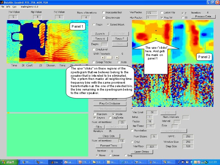
Two Speakers Semi-Supervised Source Separation.
After modeling the input signal, the user "clicks" on
those regions of the spectrogram that he believes
belong to the speaker that is intended to be eliminated.
The system then masks all neighboring
time-frequency bins with the same prominent transformation
as the one of the selected bin, the bins
remaining in the spectrogram belong to the other speaker.
Figure 13, depicts an instance of this
application. Part a) shows the user "clicks" on the spectrogram;
b) shows where the "clicks" map
into the harmonics transformation map, part c) shows
the resultant mask.
a)
b)
c)
Figure 13
Description of Video 9.
This video shows the how the demo generates the example
in figure 13.
VIDEO 9.- Two Speakers Semi-Supervised Source Separation.
CLICK ON THE SCREEN TO ACTIVE THE
VIDEO !
Missing data interpolation and Harmonics/Formants Separation.
Check videos 2, 3, 5 and 6 for examples of these applications.
Features for Speech Recognition.
The phonetic distinctions at the basis of speech recognition
reflect vocal tract filtering of glottal
excitation. In particular, the dynamics of formants (vocal
tract resonances) are known to be
powerful "information-bearing elements" in speech. We
believe the formant transformation
maps may be a robust discriminative feature to be use
in conjunction with traditional features in
speech recognition systems, particularly in noisy conditions,,
given that the belief propagation
algorithm "inforces" a dynamic structure on the transformation
maps, since often the structure
of the speech signal is higher than the noise one, the
belief propagation algorithm finds
transformation maps that are consistent with the dynamics
of the speech rather than the one of
the noise. An example of the robustness of the formants
transformation map to noisy can be
observed in figure 14, where the formant transformation
maps for a clean and noisy versions
of the same signal are shown.

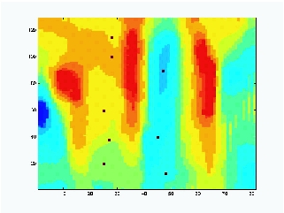
VII.- Potential Unsupervised Source Separation Application.
The right hand of figure 15, illustrates the entropy
of the distribution inferred by the system
for each tranformation variable on a composed signal.
The third pane on the figure shows
"entropy edges", boundaries of high tranformation uncertainty.
With some exceptions, these
boundaries correspond to transitions between silence
and speech, or when occlusion between
speakers starts or end. Similar edges are also found
at the transitions between voiced and
unvoiced speech. high entropy at these points indicates
that the model does not know what to
track and cannot find a good transformation to predict
the following frames. These "transition"
points are captured by the state variables, when composed
signals are modeled using the
matching-tracking model, the state nodes normally capture
the first frame of the "new
dominant" speaker, the third pane on the figure also
shows the frames chosen as states by
the system.
The source separation problem can be addressed as follows:
When multiple speakers are
present, each speaker will be modeled in its own layer,
further divided into harmonics
and formants layers. the idea is to reduce the transformation
uncertainty at the onset of
occlusions by continuining, the tracking of the "old"
speaker in one layer st the same time
as estimating the initial state of the "old" speaker
in another layer -- a realization of the
"old-plus-new" heuristic from psychoacoustics. This is
part of our current research.
Description of Video 10.
In this video, the matching-tracking model is applied
on the composed signal from figure 15.
The demo displays information in 4 panels. Panel 1, displays
the signal to
be modeled. Panel 4 displays the means set for the states
of variable St; Panel 2 displays the mean
of the most likely state for each frame; Panel 3 shows
the values of the posteriors for Ct = 1;
i.e. the probability that the model matchs frame t with
a state from variable St, rather than tracking,
(estimating) the frame from its context.
The video screen shot shows the chosen frames once the
estimation of the model parameters
is done, we edit the scrren shots with black lines to
better identify the chosen frames in the
composed signal, showing that the chosen frames have
the previously mentioned characterisitcs.
VIDEO 10.- Matching-Tracking Model on composed signals.
CLICK ON THE SCREEN TO ACTIVE THE
VIDEO !
