Homework 5

• Matlab Code

35 dB Noise		25 dB Noise

Sobel Operator

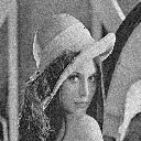
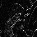
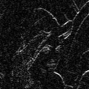
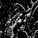
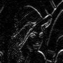
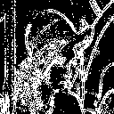
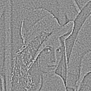
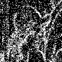
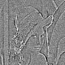
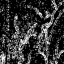
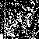
The Sobel operator is a first-order gradient operator that can be used to find the magnitude and the angle of the gradient at each point in the image. It uses two filters that find the derivative in two orthogonal directions, and uses geometry to deduce the gradient. An edge map can be created from the gradient by thresholding the gradient magnitude. Usually, the threshold is set such that a desired percentage of pixels are labelled as edge points. The figure below shows the gradient magnitudes on top, and the edge maps on the bottom, for several different threshold settings (2%, 5%, 10%, 15%) for each of the two test images (25dB noise and 35dB).

Gradient		2% Edge		5% Edge		10% Edge		15% Edge
Figure . Gradients and Edge maps using several threshold settings (2,5,10,15%). Top row: 35 dB noise, bottom: 25 dB.

For the 35dB image, 10% edge pixels looks good, but still would need post- processing before use in an object classification or similar task. Boundary linking or morphological processing could be used to clean it up. For the 25dB case, 10% is too noisy, 5% looks better.

Laplacian Operator

If the edges aren't as abrupt, then the Sobel detector might miss them. Second-order derivates may be a better place to look for edges. That's the idea behind the discrete Laplacian operator. Smoother edges may occur naturally, or they may be an artifact of an earlier smoothing process, such as a spatial average filter to remove noise. Once the image has been smoothed, a first-order edge detector like the Sobel operator may have trouble finding edges. In fact, for Lenna with a 2x2 spatial average filter, the Sobel operator still does pretty well. For a 3x3 smoothing filter, the edges start getting too thick, and we lose more gradual edges.

No smoothing		2x2 smoothing		3x3 smoothing
Figure . Sobel detectors on smoothed images. (Gradient Magnitude on top, Edge Map on bottom.)

There are several different ways to implement a discrete version of the Laplacian. The results of using the three variants shown in table 9.4 are presented below. The original image was the 35 dB image, smoothed with a 2x2 spatial average filter. The edge maps below were thresholded so that 20% are edge pixels.

L1		L2		L3
Figure . Gradients (top) and Edge maps (bottom) using the three discrete Laplacians defined in Table 9.4.

These are pretty good. The LPF has taken out most of the noise, and the Laplacian operator is able to recover the edges even though they've been smoothed. You can see, at least in the gradient if not in the edge map itself, how it picks up more gradual edges, for instance the soft edge running vertically along the whole left side of the image, which doesn't even show up in the sobel gradient at all.

It appears that for this kind of image, Laplacian 2 gives the best results. This version is defined as

[ -1 -1 -1
  -1  8 -1
  -1 -1 -1 ],

There are two complications when thresholding the laplacian gradients to get the edge map. The output of the laplacian contains both positive and negative values because the second derivative is negative in regions of downward curvature. Edge locations are actually at the inflection points, where curvature switches sign (zero crossing of the laplacians). However, for this assignment, we just threshold the absolute value of the laplacian, which gives edge points on both positive and negative extremes that exceed the threshold. Hence the double edges.

It would seem then, that since we have two edge pixels per "true edge", if we want to get comparable performance to the Sobel detector, we should set the threshold lower so that we get twice the number of pixels in the edge map as with the single-pixel-per-edge Sobel detector. And in fact, as we see in the table below, 20% edge pixels seems to be the best. The table shows various threshold percentages, using L2 on the 2x2 smoothed version of 35 dB Lenna.

10%		20%		30%
Figure . Edge maps using 10%,20%,30% edge pixels.

Actually, although the 30% edge map is messy, it picks up quite a lot of useful stuff, and it would probably be a powerful edge detector to use in a practical situation, you'd just have to do some post-processing to clean it up.

Gradient		10%		20%		30%
Figure . Laplacian edge maps and gradients of 25dB image. Top: 2x2 LPF, Bottom: 3x3.

The laplacian operator's sensitivity to noise is apparent even at 10% edge pixels. 20% would probably be usable with some good post-processing. The heavier smoothing improves the image a little bit, but not much.