Lab 4 — Large Vocabulary Decoding: A Love Story
EECS E6870: Speech Recognition
Due: Monday, December 3, 2012 at 11:59pm
- Table of Contents
- 1. Overview
- 2. Part 1: Play With FSM's and the IBM FSM Toolkit
- 3. Part 2: Investigate the Static Graph Expansion Process
- 3.1. The Model
- 3.2. Graph Expansion Steps
- 4. Part 3: Implement the Viterbi Algorithm, Handling Skip Arcs and Token Passing
- 4.1. Not Storing the Whole Chart
- 4.2. Handling Skip Arcs
- 4.3. Token Passing
- 5. Part 4: Add Support for Beam Pruning and Optionally Rank Pruning
- 5.1. Beam Pruning
- 5.2. Rank Pruning
- 6. Part 5: Evaluate the Performance of Various Models on WSJ Test Data
- 7. What is to be handed in
1. Overview
By far the sexiest piece of software associated with ASR is the large-vocabulary decoder. Since this course is nothing if not about being sexy, this assignment will deal with various aspects of large-vocabulary decoding. In the first portions of this lab, we will investigate the various steps involved in building static decoding graphs as will be needed by our decoder. In the second half of the lab, you will implement most of the interesting parts of a real-time large-vocabulary decoder. In particular, you will need to re-implement the Viterbi algorithm from Lab 2, except this time you will need to worry about memory and speed considerations as well as skip arcs. This will involve implementing token passing and beam pruning, and optionally rank pruning.
The goal of this assignment is for you, the student, to gain a better understanding of the various steps involved in constructing a static decoding graph for LVCSR and of the various algorithms used in large-vocabulary decoding. The lab consists of the following parts:
Part 1: Play with FSM's and the IBM FSM toolkit
Part 2: Investigate the static graph expansion process
Part 3: Implement the Viterbi algorithm, handling skip arcs and token passing
Part 4: Add support for beam pruning and optionally rank pruning
Part 5: Evaluate the performance of various models on WSJ test data
All of the files needed for the lab can be found in the directory /user1/faculty/stanchen/e6870/lab4/. Before starting the lab, please read the file lab4.txt; this includes all of the questions you will have to answer while doing the lab. Questions about the lab can be posted on Courseworks (https://courseworks.columbia.edu/); a discussion topic will be created for each lab.
2. Part 1: Play With FSM's and the IBM FSM Toolkit
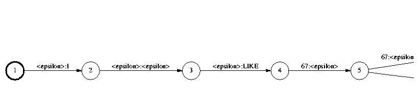
In this part, we introduce the IBM FSM toolkit as a first step in learning more about the static graph expansion process. In particular, you will be using the program FsmOp, which is a utility that can perform a variety of finite-state operations on weighted FSA's and FST's. The program FsmOp is like a calculator that operates on FSM's rather than real values, where arguments are input using reverse Polish notation as is used in some HP calculators. For example, to compute the composition of an FSA held in the file foo.fsm and an FST held in bar.fsm, you would use the command
FsmOp foo.fsm bar.fsm -compose > result.fsm |
-compose,
-determinize, and -minimize among many others.
By default, the resulting FSM is written to standard output, but
if the last argument supplied is a filename (rather than an operation),
the resulting FSM will be written to that file instead. Thus, the command
FsmOp foo.fsm bar.fsm -compose result.fsm |
We explain the default FSA format through an example:
1 2 foo 1 2 bar 2 3 moo 3 |
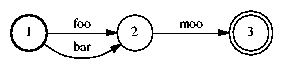
FsmOp foo.fsm -draw | dot -Tps > foo.ps |
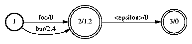
For weighted FSA's, each line can optionally be followed with a cost, or negative log probability base 10. If a cost is omitted on a line, it is taken to be zero. For example, here is a weighted FSA:
1 2 foo 1 2 bar 2.4 2 3 <epsilon> 2 1.2 3 |
Finite-state transducers have a similar format, except lines representing arcs have an extra field:
src-state dst-state in-label out-label [optional-cost] |
# transducer: true |
# transducer: true 1 2 ax AX 1 2 bar BAR 1.0 2 3 moo <epsilon> 2 1.2 3 |
For this part of the lab, you will have to create various FSM's and perform operations on them, as described in lab4.txt. Here are some hints:
Don't forget to add final states to your FSM's! Without these, your FSM's will be equivalent to empty FSM's.
For transducers, don't forget the line “# transducer: true”!
For a list of all of the operations that FsmOp can perform, run FsmOp with no arguments.
mkdir -p ~/e6870/lab4/ chmod 0700 ~/e6870/ cd ~/e6870/lab4/ cp -d /user1/faculty/stanchen/e6870/lab4/* . |
-d flag with cp (so the symbolic
links are copied over correctly).
3. Part 2: Investigate the Static Graph Expansion Process
In this part of the lab, we will look at the static graph expansion process used to create the decoding graphs that we will need for our decoder. First, we introduce the models that we are using in this lab, and then we go step-by-step through the graph expansion process.
3.1. The Model
For this lab, we will be working with the Wall Street Journal corpus. This corpus was created many years ago for a program sponsored by DARPA to spur development of basic LVCSR technology, and this corpus was designed to be about as easy as an LVCSR corpus could be for ASR. The data consists of people reading Wall Street Journal articles into a close-talking microphone in clean conditions; i.e., there is little noise. Since the data is read text, there are few conversational artifacts (such as filled pauses like UH) and it is easy to find relevant language model training data.
We trained an acoustic model on about nine hours of Wall Street Journal audio data and a smoothed trigram language model on 23M words of WSJ text. The acoustic model is context-dependent; phonetic decision trees were built for each state position (i.e., start, middle, and end) for each of the ~50 phones, yielding about 3*50=150 trees. The trees have a total of about 400 leaves; i.e., the model contains 400 GMM's, one for each context-dependent variant of each state for each phone. There are a total of about 28000 Gaussians in the model, so each GMM has about 70 components on average. The model was trained using the Attila speech recognition toolkit at IBM by first training a (1 Gaussian per GMM) context-independent phonetic model; doing several rounds of mixture splitting; growing a decision tree; seeding the CD model from the CI model; and doing a few more rounds of mixture splitting (with lots of iterations of Forward-Backward or Viterbi EM training interspersed). The vocabulary contains about 21000 words and includes all of the words in our test data (so we don't have to worry about errors caused by out-of-vocabulary words). Since our vocabulary size is about three orders of magnitude larger than in our previous decoding experiments, we use a “better” front end than the one from Lab 1 to try to get reasonable performance. In particular, the front end is a PLP front end with cepstral mean subtraction and linear discriminant analysis (to be described in later lectures). If this paragraph meant nothing to you, you should probably cut down on the brewski's.
3.2. Graph Expansion Steps
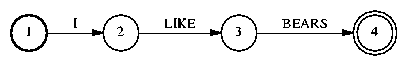
We explain the steps in graph expansion by going through an example. For full-scale decoding, we would start with a word FSM representing a pruned trigram LM; in this example, we start with a word graph wd.fsm containing just a single word sequence:
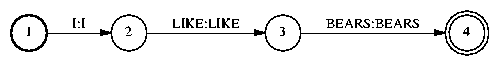
The first thing we do is convert the FSA into an FST:
FsmOp wd.fsm -make-transducer wd2.fsm |
Then, we compose the FST wd2lx.fsm to convert from words to pronunciation variants, or lexemes in IBM terminology:
FsmOp wd2.fsm wd2lx.fsm -compose lx.fsm |

Next, we convert from lexemes to phones:
FsmOp lx.fsm lx2pn.fsm -compose pn.fsm |

Next, we compose with the transducer pn2md.fsm to convert from phones to what we'll call the model level (held in the file md.fsm).
FsmOp pn.fsm pn2md.fsm -compose md.fsm |

The contents of each decision tree can be found in the file tree.txt. Here is the tree for the last state of the phone AY:
node 0: quest-P 40[+1] --> true: node 3, false: node 1 quest: AO AXR ER IY L M N NG OW OY R UH UW W Y node 1: quest-P 16[+1] --> true: node 4, false: node 2 quest: B BD CH D DD DH F G GD HH JH K KD M N NG P PD S SH TS Y node 2: quest-P 12[+1] --> true: node 5, false: node 6 quest: AO AW AX AY B BD D DD DH EH EY IH K KD M N S TS UH V W Z node 3: leaf 71 node 4: leaf 72 node 5: leaf 73 node 6: leaf 74 |
Let us go through the example of calculating the leaf number for the last state in the first AY phone in our example. Here, the phone to the right of the first AY is the “L” phone, so the question at the root node is true and we go to node 3. Node 3 contains leaf 71 and we are done.
Anyway, back to our graph expansion example. In the last step, we expand the FSM to the final HMM, rewriting each model token by the HMM that represents it:
FsmOp md.fsm md2hmm.fsm -compose -invert hmm.fsm |
The actual Gaussians parameters and mixture weights are held in the files wsj.gs and wsj.ms. These are stored in Attila's binary format, but hold the same information as the GMM parameter files we used in Lab 2. The reason we use Attila format here is because we will be calling the Attila library to do fast GMM probability computation. Attila implements a technique known as hierarchical labeling where only the probabilities of the likeliest GMM's at each frame are computed exactly; the remaining GMM's are assigned a default probability.
So, this pretty much describes all the data that we need to feed into our decoder. As mentioned before, in real life we begin with a word graph representing an n-gram language model. One of the language model graphs we use in this lab can be found in small_lm.fsm; it is a trigram model that has been pruned to about 36k bigrams and 6k trigrams. The final expanded decoding graph can be found in small_graph.fsm. It contains about 550k states and 1.3M arcs.
For this part of the lab, you will have to edit some of the FSM's used in our toy example to handle a new word in the vocabulary. In addition, you will need to do some manual decision-tree expansion; see lab4.txt for directions.
4. Part 3: Implement the Viterbi Algorithm, Handling Skip Arcs and Token Passing
In this part of the lab, you will need to re-implement the Viterbi algorithm from Lab 2, except this time handling skip arcs (i.e., arcs with no output) and token passing. We'll be doing this in three stages: first, we'll get Viterbi working without skip arcs and token passing; then we'll add skip arcs; and then we'll add token passing. For testing, we will be using isolated digit models as in Lab 2.
4.1. Not Storing the Whole Chart
Below is a pseudocode representation of the Viterbi algorithm we implemented for Lab 2:
C[0, start].logProb = 0
for t in [0 ... (T-1)]:
  for s_src in [0 ... (S-1)]:
    for a in outArcs(s_src):
      s_dst = dest(a)
      srcLogProb = C[t, s_src].logProb + a.logProb + gmmLogProb(a, t)
      if srcLogProb > C[t+1, s_dst].logProb:
        C[t+1, s_dst].logProb = srcLogProb
        C[t+1, s_dst].trace = a
|
Instead of storing the whole chart, we're only going to store the cells that we actually “visit”, where we may not visit a cell because it's not reachable from the start state or, more typically, because of pruning (which we won't actually do until the next part). We'll call the cells we visit at a frame the active cells in that frame. Another optimization we mentioned in Lecture 9 is that we don't need to keep around cells from past frames if we have some other way of recovering the best word sequence, e.g., token passing. What this boils down to is that at any point, we're only going to need to store cells from two frames, the current frame we're processing and the next frame.
To store all of the active cells at a particular frame,
we'll use a FrameData object. This structure holds
a list of FrameCell objects. These classes are documented at:
http://www.ee.columbia.edu/~stanchen/fall09/e6870/classlib/classFrameCell.html http://www.ee.columbia.edu/~stanchen/fall09/e6870/classlib/classFrameData.html |
FrameData objects, curFrame
and nextFrame, to hold active cells for the current
and next frames, respectively (frames t and t+1 in the pseudocode).
At the end of processing each frame, we copy all the cells in
nextFrame to curFrame and then clear
nextFrame at the start of the next frame,
thus setting us up correctly for the next iteration.
Looking at the pseudocode, we need to make two main changes.
First, instead of looping through all states, we
should loop through only those states with active cells
in curFrame. To do this,
we can use the methods reset_iteration() and
get_next_state(); an example of this is provided
in the code. Secondly, we need to be able to
look up the source cell C[t, s_src]
in curFrame; and
to look up the destination cell C[t+1, s_dst]
in nextFrame,
creating it if it doesn't exist. To look up the source
cell (which we already know exists), we can use
the method get_cell_by_state().
To look up the destination cell and create it if doesn't exist, we
can use the method insert_cell(). Again,
examples are provided in the code.
Your job in this part is to fill in the Viterbi algorithm
in the sections between the
markers BEGIN_LAB and END_LAB
in the file lab4_vit.C (or
Lab4Vit.java for Java).
For now, you don't have to worry about skip arcs
and you don't have to worry about computing the
correct word tree node index in each FrameCell
(just use the value 0 for now).
Read this file to see
what input and output structures need to be accessed.
We have provided sample skeleton code that you should
use as a starting point. Note: don't forget to apply
the acoustic weight!
To compile this program, type make lab4_vit, which
produces the executable lab4_vit.
(For things to work, your LD_LIBRARY_PATH environment
variable needs to be set correctly, but this should already be OK
if you set up your account correctly at the beginning of the course.)
For Java, compile via make Lab4Vit,
which produces the file Lab4Vit.class.
This program does the exact same thing as lab2_vit,
except using our new Viterbi implementation.
In particular, it first loads in a big HMM graph to use for
decoding and the associated GMM parameters. Then, for
each acoustic signal, it runs the front end to
produce feature vectors, then runs Viterbi, and then
outputs the word sequence returned by Viterbi.
For testing, we'll use the same decoding graph and GMM's that we used in Lab 2 for isolated digit recognition. To run lab4_vit (or Lab4Vit.class if lab4_vit is absent) on a single isolated digit utterance, run the script
lab4_p3a.sh |
The instructions in lab4.txt will ask you to run the script lab4_p3b.sh, which runs the decoder on a test set of ten single digit utterances.
4.2. Handling Skip Arcs
In this stage, we'll be adding support for skip arcs, or arcs with no associated GMM that don't consume a frame of input. The hard part of handling skip arcs is making sure you visit states in the correct order. As discussed in Lab 2, at a given frame, you must always visit the source state of a skip arc before its destination state for Viterbi to work correctly. One way to assure this is to renumber the states in the graph such that all skip arcs go from lower-numbered states to higher-numbered states (which will be possible as long as there are no skip arc loops), and then to visit states in increasing numeric order.
Luckily, we've done the hard work for you. We've
renumbered the states in our decoding graphs to satisfy
the preceding constraint. Also, the method
get_next_state() used to loop through cells
at a frame does indeed iterate through states
in increasing order.
In particular, it keeps track of all cells not yet iterated
through and always returns the cell corresponding to
the lowest-numbered state. In case you're interested,
the data structure we use for doing this is a
heap.
(This is tricky, because we have to be able to
handle new cells being inserted into the current frame
as we're looping through the cells in the current frame.)
However, there's still a little work left to be done for
skip arcs to work correctly, and that's your mission in
this stage of the lab. That is, you need to
edit the code you wrote for the last stage to handle
skip arcs. This should involve only changing a few
lines of code. (FYI, an arc is a skip arc if hasGmm
is false.) In particular, here are the issues you
need to address:
The location of the destination cell for a skip arc is different. (Which frame?)
When computing the log prob of the destination cell of a skip arc, there's no GMM log prob to add in.
You need to process skip arcs for when frmIdx == frmCnt (and not process non-skip arcs). One thing to worry about is that the backtrace function expects cells for the final frame to be located in
curFrame, notnextFrame. If you do this part in the way that we expect, this should happen naturally. If you don't, you may need to call
right before the backtrace function is called (and before that last call tocurFrame.swap(nextFrame);
copy_frame_to_chart()).
For testing, we'll use the same decoding graph and GMM's as in the last stage, except we've inserted some skip arcs into the decoding graph. To run lab4_vit (or Lab4Vit.class if lab4_vit is absent) on a single isolated digit utterance using this graph, run the script
lab4_p3c.sh |
4.3. Token Passing
From the previous stages, we (hopefully) now have code that can correctly compute the Viterbi probability of an utterance, even when there are skip arcs. However, we don't currently have a way to recover the word sequence labeling the Viterbi path. In this stage, we remedy this problem. Again, we will be editing your code from the previous stage.
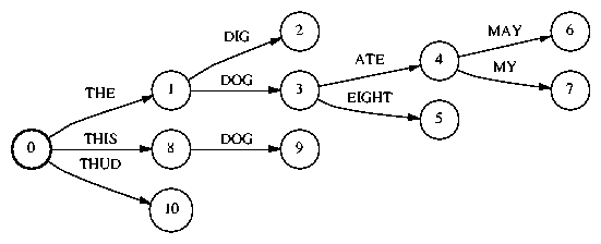
To do this, we will be constructing what we call a word tree
(which is an instance of a trie).
An example word tree is depicted in Figure 1. It can be
viewed as a way of compactly storing a list of related word sequences.
The word sequence associated with a node is the sequence of words
labeling the path from the root node to that node.
For example, in Figure 1, the index 4 corresponds to
the word sequence THE DOG ATE. We represent a word tree
using the class WordTree:
http://www.ee.columbia.edu/~stanchen/fall09/e6870/classlib/classWordTree.html |
During decoding, we will be constructing a single word tree,
stored in the variable wordTree that we declare for you.
Initially, this tree consists of a single node, the root node.
In each FrameCell, we store the index of a node
in this tree, and our goal is to do this such that the
node index at a cell corresponds to the word sequence that labels
the best path to that cell. If we do this correctly, we
can recover the best overall word sequence by finding the
word sequence associated with the best final state at the final frame.
So, how do we do this? Here are some hints.
All you have to do for this part is to correctly set the word tree node index for each cell (in addition to its Viterbi log probability, which already should be set correctly). Then, the traceback function we provide can recover the final word sequence.
Word labels occur on arcs. To find the index of the word label associated with an arc arc, do arc.get_word(). If this value is 0, then the arc has no word label. Note: most arcs do not have word labels on them.
The best word sequence for the cell associated with the start state at frame 0 is the empty word sequence. This corresponds to the root node of the word tree, or wordTree.get_root_node().
If processing an arc with no word label at a particular frame, how does the best word sequence to its destination state along that arc compare with the best word sequence to its source state?
If processing an arc with a word label at a particular frame, how does the best word sequence to its destination state along that arc compare with the best word sequence to its source state?
To find the index of the node reached by extending the node srcWordTreeIdx with the word wordIdx, do something like:
If the node doesn't exist, it will be created. For example, wordTree.insert_node(4, nextWord) would return the value 7 in Figure 1 ifint dstWordTreeIdx = wordTree.insert_node(srcWordTreeIdx, wordIdx);
nextWordcorresponds to the word MY. By doing calls like this, nodes of the word tree can be be created as needed during decoding.
Your mission for this stage of the lab is to update the code you wrote for the last stage to do token passing. You should only need to write a few lines of code for this part. For testing, we'll use the same decoding graph and GMM's as in the last stage. To run lab4_vit (or Lab4Vit.class if lab4_vit is absent) on a single isolated digit utterance using this graph, run the script
lab4_p3c.sh |
The instructions in lab4.txt will ask you to run the script lab4_p3d.sh, which runs the decoder on a test set of ten single digit utterances.
5. Part 4: Add Support for Beam Pruning and Optionally Rank Pruning
5.1. Beam Pruning
In the first task for this part, you need to implement beam pruning. Here is the general idea: before you process the outgoing arcs of a state in the main loop in Viterbi, you first check whether its log probability is above a threshold log probability, and if not, you skip that state. The threshold log probability is computed by taking the highest log probability of any cell at that frame and subtracting the beam width.
However, it is unacceptable for this lab to add any loops to compute the highest log probability at a frame, since the whole point of beam pruning is to make things faster. Instead, you must do this computation within existing loops. To complete this part of the lab, you should only have to add a few lines of code.
Again, you'll be modifying your code from earlier in this lab to complete this part. For testing, we'll use the same decoding graph and GMM's as in the last stage. To run lab4_vit (or Lab4Vit.class if lab4_vit is absent) on a single isolated digit utterance using this graph, run the script
lab4_p4a.sh |
The instructions in lab4.txt will ask you to run the script lab4_p4b.sh, which runs the decoder on a 10-sentence WSJ test set using several different beams.
5.2. Rank Pruning
This part is optional.
In this part, you can implement rank pruning. This is the same as beam pruning except that we compute the threshold in a different manner. If the rank pruning beam is set to k cells/states, we set the threshold to be the log prob of the cell in the current frame with the k-th highest log prob. In this way, we will process at most k cells at each frame (not counting the effect of skip arcs). (If there are fewer than k active cells at a frame, then rank pruning shouldn't prune away anything at that frame.) To combine rank pruning with beam pruning, just compute thresholds separately for each and use the threshold that is higher.
Unlike for beam pruning, you will probably need to add a loop. Here is an example of how to efficiently loop through all of the active cells at the current frame:
int cellCnt = curFrame.size();
for (int cellIdx = 0; cellIdx < cellCnt; ++cellIdx)
    {
    const FrameCell& curCell = curFrame.get_cell_by_index(cellIdx);
    double curLogProb = curCell.get_log_prob();
    ...
    }
|
get_next_state() since we don't need
to loop in sorted state order.)
It's OK to not keep exactly k cells at each frame
(e.g., if you do a bucket sort). For this part of the
lab, speed matters.
Again, you'll be modifying your code from earlier in this lab to complete this part. Make sure not to break the earlier parts when you do this. In particular, if k (i.e., beamStateCnt) is set to 0, turn off rank pruning. For testing, we'll be using a 10-sentence WSJ test set. First, get a baseline timing by running:
lab4_p4c.sh |
lab4_p4d.sh |
6. Part 5: Evaluate the Performance of Various Models on WSJ Test Data
In this section, we will be using the decoder you have written to run various experiments on WSJ data. We will investigate the effects of pruning and vary language model size and vocabulary size. First, if you're running C++, make sure to recompile with optimization, like so:
make clean OPTFLAGS=-O2 make lab4_vit |
Then, all you have to do in this part is run:
lab4_p5.sh | tee p5.out |
For the WSJ runs, we use the acoustic model described in Section 3.1. We consider two vocabulary sizes: the full 21k-word vocabulary, and a smaller 3k-word vocabulary (that still contains all of the words in the test set). We also consider two language models. Both are entropy-pruned versions of a modified-Kneser-Ney-smoothed trigram model built on 23M words of WSJ text. The larger LM was pruned to about 370k n-grams while the smaller LM contains a total of about 60k n-grams. For the WSJ runs, we will be using a small 10-sentence test set.
In the first set of contrast runs, we look at how the width of the pruning beam affects speed and accuracy. For these runs, we use the smaller vocabulary and LM with several different beam widths. In the next set of runs, we look at the effect of increasing vocabulary size and increasing LM size, by running with both the smaller and larger WSJ vocabularies and LM's. Look at how both speed and accuracy vary with graph size. The reference transcript for the WSJ test set can be found in wsj.ref. Check out how similar the decoded output is to the target text, and see whether you can basically understand what is being said from the decoded output.
In the final set of contrast runs, we look at the difference in the fraction of decoding time used for front end signal processing, GMM probability computation, and Viterbi search in small vs. large vocabulary tasks. For the small vocabulary run, we do an isolated digit recognition run, and for the large vocabulary run, we do WSJ with the full vocabulary and large LM. In fact, this is not a fair comparison because in the large vocabulary run, we do two things differently. Instead of doing signal processing in lab4_vit, we used Attila to produce the final feature vectors ahead of time and just read in these features directly. Secondly, as mentioned before, we use a different GMM probability computation implementation, involving hierarchical labeling and using the CBLAS math library. Despite these differences, the relative fraction of time spent on each subcomputation is still approximately correct.
If you made it this far, congratulations! You have now written most of a real-time (or close to real-time) large-vocabulary continuous speech recognizer and have shown that it works reasonably well on a (kind of) real-life task! Yay!
7. What is to be handed in
You should have a copy of the ASCII file lab4.txt in your current directory. Fill in all of the fields in this file and submit this file using the provided script.