4. Part 3: Implement Witten-Bell smoothing
Witten-Bell smoothing is this smoothing algorithm that was invented by some dude named Moffat, but dudes named Witten and Bell have generally gotten credit for it. It is significant in the field of text compression and is relatively easy to implement, and that's good enough for us.
Here's a rough motivation for this smoothing algorithm: One of the central problems in smoothing is how to estimate the probability of n-grams with zero count. For example, let's say we're building a bigram model and the bigram wi-1 wi has zero count, so PMLE(wi | wi-1) = 0. According to the Good-Turing estimate, the total mass of counts belonging to things with zero count in a distribution is the number of things with exactly one count. In other words, the probability mass assigned to the backoff distribution should be around N1(wi-1) / ch(wi-1), where N1(wi-1) is the number of words w' following wi-1 exactly once in the training data (i.e., the number of bigrams wi-1 w' with exactly one count). This suggests the following smoothing algorithm
where lambda is set to some value so that this probability distribution sums to 1, and Pbackoff(wi) is some unigram distribution that we can backoff to.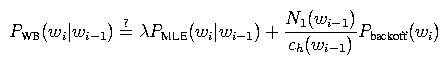
However, N1(wi-1) is kind of a finicky value; e.g., it can be zero even for distributions with lots of counts. Thus, we replace it with N1+(wi-1), the number of words following wi-1 at least once (rather than exactly once), and we fiddle with some of the other terms. Long story short, we get
For the backoff distribution, we can use an analogous equation: The term ch(epsilon) is the 0-gram history count defined earlier, and N1+(epsilon) is the number of different words with at least one count. For the backoff distribution for the unigram model, we use the uniform distribution Punif(wi) = 1 / |V|. Trigram models are defined analogously.
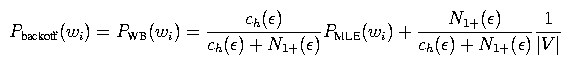
If a particular distribution has no history counts, then just use the backoff distribution directly. For example, if when computing PWB(wi | wi-1) you find that the history count ch(wi-1) is zero, then just take PWB(wi | wi-1) = PWB(wi). Intuitively, if a history h has no counts, the MLE distribution PMLE(w | h) is not meaningful and should be ignored.
Your job in this part is to fill in the function
get_prob_witten_bell(). This function should
return the value
PWB(wi | wi-2 wi-1)
given a trigram wi-2 wi-1 wi.
You will be provided with all
of the relevant counts (which you computed for Part 1).
Again, this routine corresponds to step (B) in the pseudocode
listed in Section 2.1.
Your code will again be compiled into the program EvalLMLab3. To compile this program with your code, type
smk EvalLMLab3 |
lab3p3a.sh |
The instructions in lab3.txt will ask you to run the script lab3p3b.sh, which does the same thing as lab3p3a.sh except on a different test set.