II.- SPECTRAL DEFORMATION MODEL
VIDEO 1.
Figure 1 shows a narrow band spectrogram
representation of a speech signal, where each
column depicts the energy content
across frequency in a short-time window, or time-frame.
The value in each cell is actually
the log-magnitude of the short-time Fourier transform.
![]()
Figure 1
Using the subscript C to designate
current and P to indicate previous, the model predicts
a patch of Nc time-frequency bins
centered at the kth frequency bin of frame t as a
``transformation'' of a patch
of Np bins around the kth bin of frame t-1.
Figure 1, shows an example with Nc
= 3 and Np = 5 to illustrate the intuition behind this
approach. The selected patch in frame
t can be seen as a close replica of an upward shift
of part of the patch highlighted in
frame t-1. This ``upward'' relationship can be captured by a
transformation matrix such as the
one shown in the figure.
The patch in frame t-1 is larger than
the patch in frame t to permit both upward and
downward motions.
The generative graphical model for a single layer is depicted in figure 2.
![]()
Figure 2: a)Graphical model; b) Graphical simplification
X nodes correspond to the observations,
and T nodes to the tranformations at each frequency
bin. At each bin, the local likelihood
potentials involve: the Nc bins used in the current frame,
the Np bins used in the previous frame
and the set of all possible transformation matrix defined
by T. Please read the paper
for complete details.
Inference is efficiently performed
via loopy belief propagations. Once the posteriors of the
transformation nodes are estimated,
we can find the "expected" transformation
maps an
appealing description of the harmonic's
dynamics, as can be observed in figure 3.
In these panels, the links between
three specific time-frequency bins and their corresponding
transformations on the map are highlighted.
Bin 1 is described by a steep downward
transformation, while bin 3 also has
a downward motion but is described by a less steep
transformation, consistent with the
dynamics visible in the spectrogram. Bin 2, in other hand,
is described by a steep upwards transformation.
![]()
Figure 3.- Tranformation Map.
DEMO INTRODUCTION
We have built a real time demo that performs a variety of applications using this model.
The user can change the different parameters
of the model on the user interfase, (Figure 4).
There are several panels and function
buttons that we will explain using different applications.
The information displayed on each
panel changes with each application.
We will present ten short videos
of
the demo for each application. Before each video we
will describe the application, the
information displayed in each panel and the functionality of
the buttons.
We first present an instance on the
demo performing basic estimation of the harmonics
transformation maps followed by a
harmonics tracking application.
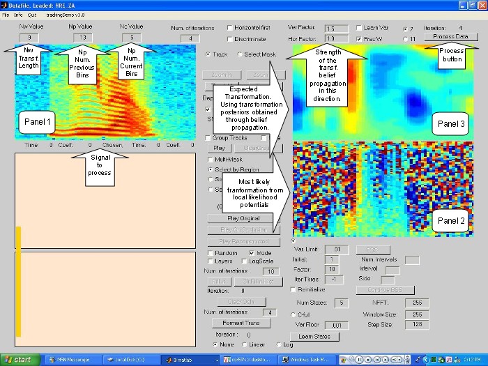
Figure 4, shows a typical "screen shot"
of the demo for this application. The figure displays
three panels. Panel 1 displays the
signal to be processed.Panel 2 shows the most likely
transformation obtained from the local
likelihood potential.Here, as in the transformations
maps,
the color relates to the motion present
in the signal, however the structure is not clearly
defined as in the transformations
maps.Also notice the total lack of a clear structure
on the
silent regions of the signal. Panel
3 shows the transformation maps obtained after each
complete iteration.
Each complete iteration consists of
complete belief propagation messages passes through all
the vertical chains.Each
vertical chain consists of all the coefficients for a given frame, followed
by the complete belief propagation
passes on all the horizontal chains, each horizontal frame
consist of all the frames for a given
coefficient.The belief propagation rules for this
chains can be
implemented using efficient forward/backward,
upward/downward recursions, see extended
paper
for details. The strength of the belief propagation in each direction is
controlled by transition
potentials in each direction. Parameters
"Ver. Factor" and "Hor. Factor" affect the probability of
switching to a different transform,
a higher value on this factor results in "smother" transformation
patterns on that direction. The video
also shows the effect of changes on thosefactors.
Once the transformation maps are estimated,
some interesting applications can be performed,
like tracking harmonics. The user
"clicks" in a certain region of the spectrogram, and if the
"Track H" button is pushed, the demo
shows the history of that particular time-frequency bin.
VIDEO 1. - Harmonics
transformations maps and harmonics
tracking application.
CLICK ON THE SCREEN TO ACTIVE THE VIDEO !