Evaluating the Z transform numerically

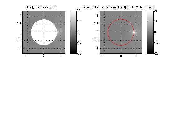
An example of actually evaluating the Z transform for different values of Z, to show what happens when you leave the region of convergence.

2011-10-06,2013-10-02 Dan Ellis [email protected]

Here, we evaluate $X(z) = \sum_n x[n] z^{-n}$ for an approximation to an indefinite-length sequence (the first 1000 points of an exponentially-decaying function) over a grid of $z$ values; this clearly reveals the region of convergence, and the rapid explosion of the evaluated $X(z)$ function when we leave the region of convergence. Of course, in this example, because we are evaluating only a finite range of n values, the function doesn't actually become infinite (although it does overflow even Matlab's 64 bit floating point representation in a few places), but it rapidly becomes so large that the trend is obvious.

Let's look at the sequence $x[n] = \mu[n] \cdot \alpha^n$ for $\alpha = 0.8$ , and over the range $n = 0\ldots 999$ (1000 points)

n = [0:999];
alpha = 0.8;
x = alpha.^n;

% By its 1000th point, x[n] has gotten quite small:
x(end)

ans =

   1.5378e-97

For a given value of $z$ , we can evaluate $X(z)$ by directly calculating the summation in the Z transform. This is the exact value of the Z transform for the finite-length $x[n]$ we are actually dealing with, but we can treat it as an approximation to the Z transform of the infinite-length $x[n] = \mu[n] \alpha^n$ The closed-form Z-transform for this sequence is, of course, $X(z) = 1/(1 - \alpha z^{-1})$ for $|z| > |\alpha|$

z = 1.0;
X = sum(x .* (z.^(-n)))    % 5.0

% (We note in passing that $z = 1.0$ is also $z = e^{j\omega}$ for
% $\omega = 0$, i.e. it is the zero-frequency value of the DTFT, and
% hence also the zero-index term of the DFT.  Check:
Xf = fft(x);
Xf(1)      % 5.0 )

X =

    5.0000


ans =

    5.0000

OK, let's evaluate $X(z)$ not just for a single value of $z$ , but for a uniform dense grid of values covering the $z$ -plane from -1.3 to 1.3 and from -1.3j to +1.3j

incr = 0.01;
zlim = 1.3;
zvals = (-zlim):incr:zlim;
for row = 1:length(zvals)
  for col = 1:length(zvals)
    z = zvals(col) + sqrt(-1)*zvals(row);
    X(row, col) = sum(x .* (z.^(-n)));
    % While we're here, also calculate the closed-form value of the
    % full (infinite)-length x, to compare
    Xc(row, col) = 1/(1 - alpha/z);
  end
end
% We're calcuating 260x260 ~= 70,000 values, so it make take a few
% seconds

% We now have a square array X(row,col) giving the values of our
% Z transform every 0.01 over the range z values from -1.3 - j(1.3)
% to 1.3 + j(1.3).
% Some values close to (0,0) exceeded the numerical resolution and
% ended up as NaNs.  Let's just set these to Inf for consistency:
X(isnan(X(:))) = Inf;
% Plot the magnitudes as a grayscale image
subplot(221)
imagesc(zvals, zvals, abs(X))
axis xy; axis square; grid
title('|X(z)|, direct evaluation')
colormap('gray')
colorbar
% Matlab is trying hard to show us some very large values, with the
% effect that nothing much is visible.  Let's limit the color range
% to some sensible values
caxis([-20 20])
% Now we can see a boundary, and a little detail near the pole at
% (0.8, 0).

% Let's compare this to the closed-form results
subplot(222)
imagesc(zvals, zvals, abs(Xc))
axis xy; axis square; grid
title('Closed-form expression for |X(z)| + ROC boundary')
colorbar
caxis([-20 20])
% overplot the ROC boundary at |z| = \alpha
omega = [0:.01:2*pi];
hold on; plot(alpha*cos(omega), alpha*sin(omega), '-r'); hold off
% We can now see that the closed-form equation does indeed give us
% the right values for X(z), but only in the region of convergence
% (the area outside the red circle).

The bottom line here is to illustrate the difference between the actual $X(z)$ calculated by literal application of the Z-transform definition, and the values given by the closed form solution (i.e., they match only in the ROC), and also to show that slightly surprising behavior of the Z-transform sum -- that $X(z)$ abruptly explodes at the edge of the ROC defined by $|z| = \alpha$ -- really does happen that way, even for a finite-length approximation to an infinite causal sequence.