Manual User’s Version 1.0
LabROSA Department of Electrical Engineering http://labrosa.ee.columbia.edu/
Introduction
The phenomena of language perception have framed and propelled much of contemporary psychology.
Psychologists have sought to understand how human listeners understand language, and more specifically how our auditory system efficiently processes language in an environment where silence is normally the exception. Speech often arrives at the ears of the listener as a rather different entity than on production. The effects of background noise, reverberation, communication channel restrictions and failures, and the presence of other sources all contribute to the degradation of the signal. Listeners possess strategies for handling many types of distortion, and uncovering these strategies is of importance in understanding speech intelligibility under noise situations, or designing robust systems for computational hearing.
But psychologists know little about signal processing, frequency components, acoustics or computer programming. That is why interdisciplinary research groups like Hoarse (www.hoarsenet.org) have emerged over the last decade. Their aim is to put together different sources of knowledge, attitudes, and skills in order to better understand our sophisticated auditory and cognitive system.
The Oreja project combines aspects of engineering and psychology to allow researchers interested in speech perception (coming from other disciplines such as phonetics, linguistics, etc.), to manipulate a speech signal, and study how these manipulations affect the percept of that signal.
Two sources inspired this software. First a
paper written by Kasturi and Loizou (2002) assessed the intelligibility of
speech where normal-hearing listeners have either a single “hole” in various
bands or have two “holes” in disjoint or adjacent bands in the spectrum. After
reading this paper I wanted to design a similar experiment, but instead of
adding holes in various bands, I chose to mask these bands with different types
of noise. I imagined an intuitive interface that would allow me to filter the
speech into different bands, select maskers from a menu of noises, and finally
hear the output by simply pressing an imaginary ‘play’ key. Software like this
does not exist. However, a second source of inspiration was found: the work
done by Cook, Brown, and Wrigley (1998) called ‘Mad’ (MATLAB auditory
demonstrations). These demonstrations exist within a computer-assisted learning
(
After exploring the versatility of Mad, investing time in a limited program was not worth it. Instead, I preferred to build a psychoacoustic tool with a wide range of possibilities and menus accessible to a large and heterogeneous group of language and speech researchers.
Raul Rodriguez-Esteban, an engineer who kindly has been collaborating in the whole project, has been the one materializing the experimental conditions in this first version of Oreja. That is how Oreja, intuitive software using MATLAB code to easily design psychoacoustic experiments, came to life.
Welcome to Oreja
Most manuals make tiresome reading. This guide aims to be as clear and helpful as possible. In this manual we are going to try to use a simple vocabulary, and if for any reason you find a technical concept that you are not familiar with, please go to the glossary for an explanation [If it is not there, contact us and we will include it in the next version of Oreja. The easiest way to contact us is by clicking in the help menu] . Our intention is not to be patronizing, instead we want to ensure that anyone interested in speech perception can use Oreja and understand, for example, how noise affects speech intelligibility, or the underlying processes that allows us to segregate noise from a speech signal.
Due to its interactive and intuitive interface, Oreja can
also be used as a
Basic idea
Oreja V.1.0 is a software that has been designed specially to study speech intelligibility. It has two main windows. The first one basically allows you to load, decompose into different channels, analyze, and select the parts of the signal you want to label and/or manipulate. Moreover, with Oreja you can load more than one signal concatenating them one after the other.
The second window has been designed to alter these signals in many different ways (e.g., attenuating the amplitude of the channels selected, or adding noise), and save them in an audio file format. Once these signals have been manipulated and saved, you can always load them again.
Basically, the first window helps you to select the speech signal, and the second one helps you to create background noises that mask the speech or transform parts of the original signal in many different ways.
There are many possibilities but lets go step by step.
How to use
Oreja
Step by step
Oreja has been
implemented using MATLAB. That means MATLAB should be installed in the computer
if you want to run Oreja. MATLAB is a high-level programming language which
provides functions for numerical computation, user interface creation and data
visualization. Oreja has been updated in 2004 for MATLAB 6.5 on Windows XP. If this is the first time you have
used MATLAB, just follow the instructions.
Installation (…)
The structure of
the Oreja directory (…)
MATLAB
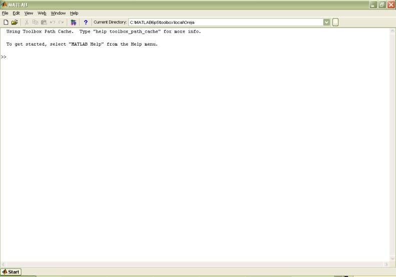
To
start Oreja type ‘oreja’ at the MATLAB prompt of the command window. Make sure
you are in the right directory and press enter, otherwise browse for the right
folder.
Type oreja

Check if you are in the right directory

Fig.1 This is the first
window you will see when opening MATLAB
|
Type oreja |
|
Check if you are in the right directory |
|
Fig.1 This is the first
window you will see when opening MATLAB |
First window: Signal
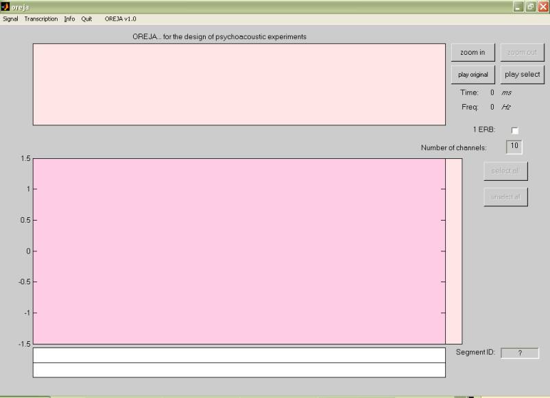
Once
you have typed oreja, a new window like the one below (fig.2) will appear on
your screen. This is the first window
of Oreja. On the top left part of this screen (1) there is a menu with the
following options: Signal, Transposition,
Info, Quit and Oreja v1.0.

Click in the signal menu to display the popup menu that will let you
load a sound file
|
Click in the signal menu to display the popup menu that will let you
load a sound file |
Fig.2 Appearance of Oreja
when no signals have been loaded.
![]()

![]()
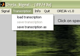
The menu signal (fig. 3) will display a popup menu with the following options: load signal, manipulate selection, concatenate signal. The load signal option will open another window called ‘new signal’. From this new window you can select the sound file you want to download. The file format of these signals should be .au, .wav, or .snd. Any other format is not supported by Oreja… yet.
Fig.3 Signal popup menu
|
Fig.3 Signal popup menu |
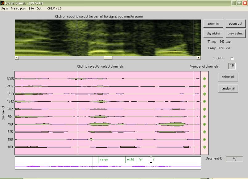
Once you have chosen and loaded a sound file, three different representations from this sound file (the one you have just selected) will appear in panel 1, 2, and 3 (see fig. 2). Panel 1 will show the spectrogram of the signal selected. The intensity of the signal will be represented in the spectrogram with green tones (light green represents more intensity or energy). In panel 2 the signal will appear filtered automatically into ten frequency channels. The selected channels will appear in green, and the unselected channels will appear in ivory. Panel 3 will represent the waveform of the sound file loaded. In all these three panels time is represented in the x axis and frequency in the y axes, which corresponds to our impression of the highness of a sound.
The name of the signal loaded (the name in which it has been saved) will appear on top of the window (2).
If you select concatenate signal from the signal menu (see fig.3), a window like the one appearing in load signal will appear in the screen. Select the sound file you want to add to the previous loaded signal. You can concatenate as many signal as you wish. You have to decide the order of the concatenated signals in advance. Oreja only allows you to put them sequentially one after the other.
Figure 4 shows you the way the loaded signal is represented.
Cursors
As you move the mouse or the cursors (shown as vertical lines) by dragging them over panel 1, the time and frequency under the current location will be shown at the top right (8).
Cursors from panel 1 and 2 are connected because both share the same time scale of the signal. However the cursors from panel 3 are only linked to the cursors from panel 1 and 2 when the whole signal is represented in the first loaded stage. It is only in this first stage that all the panels represent the whole signal. Another difference between these three panels is that the portion of the signal between the cursors will be played back if you click on top of the waveform of panel 3. This property will help you to accurately select the segment of speech you wish to manipulate.
The main goal of this first window is to allow the user to select precise portions of the signal by frequency domain using panels 1 and 2, or time domain using panel 3.
The spectrogram display has linear-in-Hz y-axis, whereas the filter center frequencies (CF) are arrayed on a ERB-rate [Equivalent Rectangular Bandwidth] scale. The latter is approximately logarithmic.
Zoom
Moving the vertical lines or cursors will facilitate the selection of the specific segment of the signal you want to manipulate. Use the zoom in and zoom out (5) buttons together with the slide bar (3) to facilitate the accuracy of the selection.
The buttons Zoom in and Zoom out only work for panel 1 and 2. In panel 3 the signal loaded will be represented completely at any time. This panel helps you to have a better perspective of the whole signal.
![]()
![]()

![]()
![]()
![]()
![]()
![]()
![]()

![]()
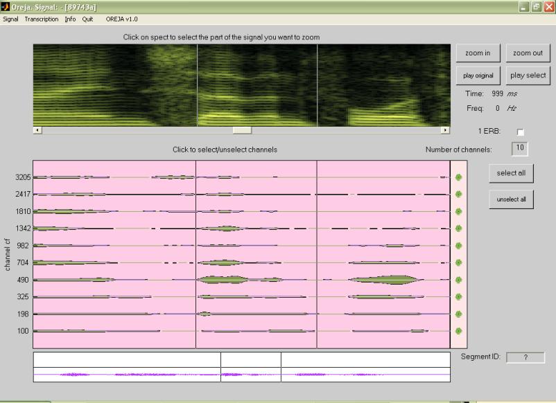
Fig.4 This is the way the
signal is represented
Channels & Filters
By default all the
channels will be selected after loading the signal. You can select different channels
by clicking on individual waveforms or on the little circles of panel 2 (12).
You can listen to these individual bands by first selecting them, and then
clicking the play selected button (6).
An unselected signal does not contribute to the overall output. By
selecting/unselecting you can explore various forms of spectral filtering and
start designing the stimuli of your experiment. Alternatively, you can use the
buttons select all/unselect all (11)
to speed up the selection process. To hear the original signal click the button
play original (7). To change the
number of channels insert another number in
Filtering means that the signal will be ‘divided’ into ten different bands or channels (ten is the default number but you can always change it). The information contained in each band depends on the filterbank applied. The filters used to divide the signal are a bank of second-order auditory gammatone bandpass filters. The center frequencies of the filters are shown on the left side of the display (4). The distance between their frequency centers is based on the ERB fit to the human cochlea. The default filterbank covers uniformly the whole signal with minimal gaps between the bands. You can change the default bandwidths by checking the box number 9, which forces all filters to have a bandwidth of 1 ERB regardless of their spacing. This option leaves larger gaps between the filtered signal bands for banks of fewer than ten bands, but the distances between the frequency centers are not changed. Notice that when filtering the signal by a small number of channels the default filterbank brings more information than the '1 ERB' filters. The suitability of each filterbank depends of the design of your experiment.
Fig.5 Divide the signal
and label its segments.
Transcription
Look now at fig. 5. Panel 4 has been created to label the signal or parts of this signal.
In order to introduce
annotations or labels, first you must select the parts of the speech you want
to label with the cursors. If you double click on one of the cursors on panel 4
it will change color, and if you click again, two little black squares will appear
at the edges of the cursors (13). Whatever you type in
A label can be deleted by selecting the object and pressing the delete key of the keyboard.
Fig.6 Load or save your transcriptions.
Once you have selected the parts of the speech signal and the channels you want to manipulate, go to the signal popup menu and click manipulate selection (fig. 3). You can always go back to this window if, for any reason, your selection is not exactly what you expected.
Info
The info menu contains a popup menu with the logo of Oreja and also this manual in html format.
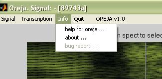
Fig.7 Info menu
Quit
Quit will close Oreja and you will go back to the MATLAB prompt.
Second window:
Manipulation
Once the selection is done choose the manipulate selection option from the signal menu (fig.3), and a second window will appear (fig.8) with all the channels you wish to manipulate represented in two panels. Panel 19 is similar to panel 2 of the first window, and panel 21 is analog to panel 1.
As in the first window you can choose different channels of the portion of the signal selected by clicking in the circles or by pressing the select all/unselect all buttons (26). In this window the cursors will help you to select the area of the signal you want to manipulate by looking at the time and frequency displays located at the top of the window (27). Select accurately the exact time portion you wish manipulate (e.g. mask with white noise a component) by using the from/to option of the general settings menu (23). As in the first window, you can specify the channels (frequency domain) you want to alter by clicking the circles.
The play button (18) plays back all the channels that appear in panel 19 regardless of whether they are selected or not. The distortion menu (24, 25) has been organize as follows; speech, tone and noises will affect to all the channels (selected or not), but will mask only the time period selected with the from/to function. However gain, time reverse, and sinewaves replicas will affect only the channels selected. For example, if you select only the lowest channel and the sine-wave replicas option (22), and then press add, only that channel will be converted into a sinusoid or narrow band. On the contrary, if you select the same channel but on this occasion you select noises (22), and from the pop up menu white noise, all channels will be affected unless you specify its duration in menu 23.
In panel 21 you can visualize the spectra of the selected portions in combination with the manipulations added. The play button 20 will play back the portion of signal selected plus the distortions added.
Fig, 8 Appearance of the
second window![]()
![]()
![]()
![]()
![]()
![]()
![]()
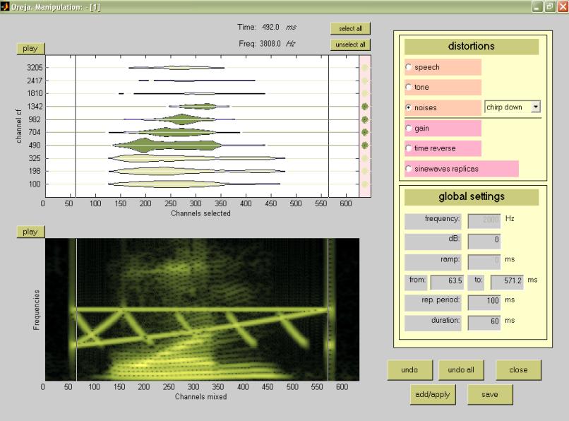
Use the distortion menu on the upper right of the screen (24, 25) to select the stimuli you want to add, subtract or apply. Notice that only the global settings that are relevant for each stimulus will be enabled. For example, if you select gain to modify the amplitude of one or several channels, only the dB box will be active because is the only value that is related to amplitude. Let’s go step by step and explore the possibilities from menu 23, 24 and 25:
Distortions
1. Adding signals
- speech: The purpose of this option is to mix the signal selected with streams of speech or other signals. Your specific inputs depend upon which kind of experiment you want to design. The advantage of this option is that you can select and manipulate a speech signal, save it on one of these files and mix it later with another signal (for example, to study the Cocktail party effect. See glossary).
- tone: Generates a sine wave tone. Choose its frequency, its duration, the starting and ending point, its ramp, and the repetition rate just in case you want to create a tone that stops and starts at a regular rate. For the moment, if you want to create a single tone that appears randomly, you must do it manually.
- noises: This menu contains five stimuli; white noise, brown noise, pink noise, chirp up, and chirp down. You can change the parameters of the stimuli chirp up, and chirp down from the code that generates them. To do this you need to close Oreja, find the file chirp_up.m or chirp_down.m and change the values of f0 and f1. For example, chirp up have been set as a swept-frequency cosine signal, where f0 is the instantaneous frequency at time 0 (1000 Hz), and f1 is the instantaneous frequency at time t1 (2000 Hz). If you want to create a chirp up that goes from 4 kHz (kilohertz) to 6 kHz, just change the values of f0 = 4000 and f1=6000. Notice that stimuli like bursts can be generated selecting a type of noise (e.g., pink noise), and setting its duration.
2. Transformations
- gain: Adjusts the amplitude of the channel selected. Accepts negative values for attenuating the selected channels.
- time reverse: Inverts the channel selected. As a result you will hear the signal backwards.
- Sine-wave replicas: Sine-wave speech is a synthetic analogue of natural speech represented by a small number of time-varying sinusoids. It sounds like a talking robot. (See glossary for a detailed definition).
global settings
- frequency: The number of wave repetitions in a periodic vibration within a fixed time period. A high number will produce high-frequency sounds, and conversely. Choose values from 0 up to half the sampling frequency, higher values will cause aliasing effects.
- dB: Abbreviation of decibel. A unit of sound intensity. It is the measure of gain in which a signal is amplified or attenuated. The decibel is a relational measure, expressing the relative intensity of the described sound to a reference sound. In Oreja the reference sound is the signal itself when using the option ‘gain’ or ‘speech’. When using the options ‘tone’ or ‘noises’ the tones and noises generated will be amplified with respect to the original signal. As baseline 0 dB is an amplitude of 10% the maximum of the original signal.
- duration: Length of the working cycle when a repetition rate is chosen. The working cycle is the part of the repetition period that includes signal.
- from/to: The starting and end point of the masker.
- ramp: Ensure that the tone marker starts and stops smoothly.
- fs: Abbreviation of sampling frequency. It is the number of times an analog signal is measured (sampled) per second. The unit of the sampling frequency is "samples per second". This is often expressed in kilohertz (kHz). For example, "CD quality" sound has a sample frequency of 44 kHz.
- rep. period: Abbreviation of repetition period. Useful when introducing a masker that appears several times masking the signal. If the frequency of appearance is constant, you just need to decide its period. However, if the frequency of appearance is random, you will need to add the maskers manually one by one.
Finally, the group of buttons situated in the right bottom part of the screen (22), will allow you to save the manipulations done, undo the last one, undo all of them, add information to the signal, or close the window. The undo button, opposite to the undo all, only undoes the last operation added. Close will close the window and you will go back to the previous one. The add button adds all the information selected from the distortion and the general settings menu. You can add more than one masker or distortion to the same signal.
Enjoy.
Acknowlegments
This project could have not been developed in LabRosa without the supervision of Dan Ellis and the Fulbright scholarship granted to one of the authors. Thanks so much to Daniel Donnelly for corrections and insightful suggestions on the first draft of this manual.
References
Bergman, A.S. (1990). Auditory Scene Analysis. MIT Press.
Cooke, M.P. and Brown, G. J. (1999). Interactive
explorations in speech and hearing. J.
Acoust. Soc.
Glasberg, B.R. & Moore, B.C. (1990). Derivation of auditory filter shapes from notched-noise data, Hearing Research. 47, 103-138.
Kasturi, K. & Loizou, P.C. (2002). The
intelligibility of speech with “holes” in the spectrum. Jounal of the Acoustical Society of
Patterson, R. D. & Holdsworth, J.
(1991). A Functional Model of Neural Activity Patterns and Auditory Images. Advances in speech, Hearing and Language
Processing, vol.3, JAI Press,
Remez, R.E., Rubin, P.E., Pisono, D.B. and Carrell, T.D. (1981). Speech perception without traditional speech cues. Science, 212, 947-950.
Remez, R. E., Rubin, P. E., Berns, S. M., Pardo, J. S., & Lang,
J. M. (1994). On the perceptual organization of speech, Psychological Review,
101, 129-156.
Glossary
Auditory stream: A
mental description of a physical (or virtual) sound source and its behavior
through time. Auditory stream segregation
refers to the process of perceptual organization of sound that accomplishes the
construction of this description.
Band-pass: Filter that allows a range of frequencies through, attenuating
those that are lower and higher than the desired band of frequencies.
Bark scale: A frequency scale on which equal
distances correspond with perceptually equal distances. Above
approximately at 500 Hz this scale is more or less equal to a logarithmic
frequency axis. Below 500 Hz the Bark scale becomes progressively more linear.
Chirp: A
short, sharp
note, as
of
a
bird or
insect. Swept-frequency cosine signal, where
f0 is the instantaneous frequency at time 0, and f1 is the instantaneous
frequency at time t1. The frequencies of a chirp up have an ascend direction
where f0 > f1. Chirp down is the same as chirp up but with f1 > f0.
Cocktail party effect: A form of auditory stream segregation by which a listener's ability to localize sound sources can increase intelligibility. So called because at a cocktail party, a listener can focus on, and understand, a conversation while dozens or even hundreds of other conversations occur all around. If a conventional 2-channel high-resolution recording were made and subsequently played back, the listener would not be able to understand individual conversations because they have been spatially blended into the two speakers.
Decibel: A unit of the intensity of sound. The decibel (abbreviated dB) is a relative measure, expressing the relative intensity of the described sound to a reference sound. The decibel is a logarithmic measure, specifically 10 times the logarithm of the ratio of two voltages, currents or sound pressures. A difference of 20 dB between two sounds means that the more intense one has 100 times the amplitude of the softer. A single decibel is commonly thought to be the smallest change in sound pressure level that the trained human ear can detect.
Envelope: The envelope of a function is a smooth
curve passing through the peaks of the function (e g. spectral envelope).
ERB-rate scale: Measuring the critical bands
below 500 Hz appeared to be quite difficult, due to the fact that, at low
frequencies, the sensitivity and the efficiency of the auditory system diminish
rapidly, while headphone technology caused leakage of acoustic energy at low
frequencies. More accurate measurements of the auditory-filter bandwidth
have now leaded to the ERB-rate scale. These measurements have used notched-noise
maskers to measure the auditory filter bandwidth. In general, on this
ERB-rate scale the auditory-filter bandwidth, expressed in equivalent
rectangular bandwidth (ERB) is smaller than on the Bark scale, a difference which becomes larger for lower
frequencies.
Filter: A device that can change the relative amplitudes and phases of the frequency components in the spectrum of a signal. A high-pass filter attenuates low frequencies and allows high frequencies pass through. A low-pass filter does the opposite.
Fourier analysis: A mathematical analysis of continuous signals, discovered by the French mathematician Fourier. He proved that any periodic, or non periodic sound of limited duration, could be represented or created with a sum of pure tones with different frequencies, amplitudes, and phases.
Frequency: The number of repetitions of the wave in a periodic vibration within a fixed time period.
Fundamental frequency: The lowest tone of a harmonic series. Its abbreviation is F0.
Gammatone filter: Auditory filter designed by Patterson (1991), and it is known to effectively simulate the response of the basilar membrane. The amplitude term represented by the Gamma distribution is
![]()
where f0 is the center frequency. The amplitude characteristics of the gammatone filter are represented approximately by
![]()
where GT(f) is the Fourier transform of gt(t) and represents band-pass filtering with a center frequency of f0.
Harmonic: Name given to a frequency component of a spectrum in which the frequency of every component is a multiple of a low frequency called the fundamental frequency.
Harmonicity: The state of being harmonic or periodic. Periodicity is mathematically synonymous with harmonicity, though the former usually refers to a regularity in the sound's time description while the latter refers to a regularity in its frequency description.
Intensity: The name given to the physical energy with which a sound is present. It contrasts with "loudness," which is the perceptual experience approximately correlated with that physical intensity.
Linear scale: Scale on which actual distances from the origin are proportional to the corresponding scale numbers.
Logarithmic scales: Scale on which actual distances from the origin are proportional to the logarithms of the corresponding scale numbers. This has the effect that equal steps along the scale represent equal ratios between the raw values (origin). Examples in audition are the decibel scale and the scale of musical pitch.
Noise: A noise waveform consists not of regular
periodic cycles but of random fluctuations of amplitude. White noise is a random waveform whose frequency spectrum
contains all audible frequencies. A noise signal that contains all frequencies
with equal energy per octave is called pink noise, commonly used to test
loudspeakers. A noise signal that is filtered, removing higher and lower
frequencies and just letting through a small band of frequencies, is called narrow-band or band-pass noise. Filtering out the high frequencies starting from
a certain cut-off frequency gives low-pass
noise or brown noise. Taking a noise
waveform over a certain time period and then repeating this segment gives what
is called frozen noise.
Octave: One of the pitch intervals in music. Physically, a note that is an octave higher than another has a frequency that is twice that of the lower one. Tones separated by an octave have an equivalent quality and are assigned the same note name (for example “C”) in western music and the same role in harmony.
Periodic: A periodic sound is one that repeats itself after a period of time. As a consequence, it can be represented as the sum of a set of harmonics using Fourier analysis. If this is not true, the sound is said to be aperiodic.
Phase: Particular point in a wave that is passing a position in space at a certain instant of time. Phase is measured in units of degrees, with 360 degrees representing one complete cycle of the wave. If two tones have the same period and are occurring at the same time, the temporal lag of one with respect the other can be described in terms of phase. If two waves are out of phase by 180 degrees, the later one is lagging by half a period.
Pure tone: A tone with only a single frequency component. Its wave form will be that of a sine-wave.
Sine wave: The simplest form of periodic wave motion, expressed by the equation y = sin (wt+p), where w is the frequency, t is the time, p is the phase and y is voltage or sound pressure level. All other forms can be created by adding (mixing) a number of sine waves. The wave form of a pure tone is a sine-wave.
Sine-waves replicas: Sine-wave speech is a synthetic analogue of the procedure of natural speech by a small number of time-varying sinusoids. Listeners perform well at transcribing sine-wave replicas of utterances (Remez et al, 1981). It has been argued that sine-wave speech demonstrates the special status of speech in auditory perception. Of late, proponents of this hypothesis have used sine-wave speech experiments (Remez et al, 1994) to suggest that speech is beyond the reach of the ‘gestalt’ grouping processes which motivate the auditory scene analysis (ASA) account of sound perception (Bergman, 1990).
Sound: Energy transmitted by pressure waves in air or other materials and that is the objective cause of the sensation of hearing. Longitudinal vibrations in a medium in the frequency range 20 Hz to 20 kHz.
Speech intelligibility: A measure of sound clarity that indicates the ease of understanding speech. It is a complex function of psychoacoustics, signal-to-noise ratio of the sound source, and direct-to-reverberant energy within the listening environment.
Spectrum: A description of the frequency content of a sound waveform, usually presented as a graph with frequency on the abscissa (x axis) and amplitude on the ordinate (y axis). A pure tone would have a single vertical line at the appropriate frequency with a height indicating its amplitude. A complex sound would have several such lines, indicating the multiple components. Drawing a curve through the tops of the lines would describe the spectral envelope.
Spectrogram: A representation of a spectrum in which the time component is reintroduced: time is represented on the abscissa, frequency on the ordinate, and amplitude is coded as the darkness/lightness of the trace at a given frequency and time. In an auditory neural spectrogram, instead of a continuous signal, the probability of occurrence of nerve spikes at a given moment in time is represented. The frequency axis is replaced by a frequency-specific auditory nerve channel. A third type of spectral representation called a time-frequency perspective plot is drawn in three dimensions, with time along the x axis, amplitude along the y axis, and frequency along the z axis.
Sinusoidal: Having the shape of a sine wave.
Glossary
references:
Bergman, A.S. (1990). Auditory Scene Analysis. MIT Press.
http://www.keithyates.com/glossary.htm#anchor604241
About the authors
Elvira Perez is
currently a Fulbright scholar at LabRosa (Dept. of Electrical Engineering at
Raul Rodriguez-Esteban
is currently a Ph.D. student in the Dept. of Electrical Engineering at