9.5 Tree-Based Clustering

 

  One limitation of the data-driven clustering procedure described above is that it does not deal with triphones for which there are no examples in the training data. When building word-internal triphone systems, this problem can often be avoided by careful design of the training database but when building large vocabulary cross-word triphone systems unseen triphones are unavoidable.  

 

HHED provides an alternative decision tree based clustering  mechanism which provides a similar quality of clustering but offers a solution to the unseen triphone problem. Decision tree-based clustering is invoked by the command TB which is analogous to the TC command described above and has an identical form, that is

    TB thresh macroname itemlist

Apart from the clustering mechanism, there are some other differences between TC and TB. Firstly, TC uses a distance metric between states whereas TB uses a log likelihood criterion. Thus, the threshold values are not directly comparable. Furthermore, TC supports any type of output distribution whereas TB only supports single-Gaussian continuous density output distributions. Secondly, although the following describes only state clustering, the TB command  can also be used to cluster whole models.

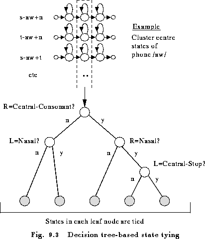
A phonetic decision tree is a binary tree in which a yes/no phonetic question  is attached to each node. Initially all states in a given item list (typically a specific phone state position) are placed at the root node of a tree. Depending on each answer, the pool of states is successively split and this continues until the states have trickled down to leaf-nodes. All states in the same leaf node are then tied. For example, Fig 9.3 illustrates the case of tying the centre states of all triphones of the phone /aw/ (as in ``out''). All of the states trickle down the tree and depending on the answer to the questions, they end up at one of the shaded terminal nodes. For example, in the illustrated case, the centre state of s-aw+n would join the second leaf node from the right since its right context is a central consonant, and its right context is a nasal but its left context is not a central stop.

The question at each node is chosen to (locally) maximise the likelihood of the training data given the final set of state tyings. Before any tree building can take place, all of the possible phonetic questions must be loaded into HHED using QS commands . Each question takes the form ``Is the left or right context in the set P?'' where the context is the model context as defined by its logical name. The set P is represented by an item list and for convenience every question is given a name. As an example, the following command

    QS "L_Nasal" { ng-*,n-*,m-* }

defines the question ``Is the left context a nasal?''.

It is possible to calculate the log likelihood of the training data given any pool of states (or models). Furthermore, this can be done without reference to the training data itself since for single Gaussian distributions the means, variances and state occupation counts (input via a stats file) form sufficient statistics. Splitting any pool into two will increase the log likelihood since it provides twice as many parameters to model the same amount of data. The increase obtained when each possible question is used can thus be calculated and the question selected which gives the biggest improvement.

Trees are therefore built using a top-down sequential optimisation process. Initially all states (or models) are placed in a single cluster at the root of the tree. The question is then found which gives the best split of the root node. This process is repeated until the increase in log likelihood falls below the threshold specified in the TB command. As a final stage, the decrease in log likelihood is calculated for merging terminal nodes with differing parents. Any pair of nodes for which this decrease is less than the threshold used to stop splitting are then merged.  

As with the TC command, it is useful to prevent the creation of clusters with very little associated training data. The RO command can therefore be used in tree clustering as well as in data-driven clustering. When used with trees, any split which would result in a total occupation count falling below the value specified is prohibited. Note that the RO command can also be used to load the required stats file. Alternatively, the stats file can be loaded using the LS command .

As with data-driven clustering, using the trace facilities provided by HHED is recommended for monitoring and setting the appropriate thresholds. Basic tracing provides the following summary data for each tree

    TB 350.00 aw_s3 {}
     Tree based clustering
      Start  aw[3] : 28  have  LogL=-86.899 occ=864.2
      Via    aw[3] : 5   gives LogL=-84.421 occ=864.2
      End    aw[3] : 5   gives LogL=-84.421 occ=864.2
    TB: Stats 28->5 [17.9%]  { 4537->285 [6.3%] total }

This example corresponds to the case illustrated in Fig 9.3. The TB command has been invoked with a threshold of 350.0 to cluster the centre states of the triphones of the phone aw. At the start of clustering with all 28 states in a single pool, the average log likelihood per unit of occupation is -86.9 and on completion with 5 clusters this has increased to -84.4. The middle line labelled ``via'' gives the position after the tree has been built but before terminal nodes have been merged (none were merged in this case). The last line summarises the overall position. After building this tree, a total of 4537 states were reduced to 285 clusters. 

As noted at the start of this section, an important advantage of tree-based clustering is that it allows triphone models which have no training data to be synthesised. This is done in HHED using the AU command  which has the form

    AU hmmlist

Its effect is to scan the given hmmlist and any physical models listed which are not in the currently loaded set are synthesised. This is done by descending the previously constructed trees for that phone and answering the questions at each node based on the new unseen context. When each leaf node is reached, the state representing that cluster is used for the corresponding state in the unseen triphone .

The AU command can be used within the same edit script as the tree building commands. However, it will often be the case that a new set of triphones is needed at a later date, perhaps as a result of vocabulary changes. To make this possible, a complete set of trees can be saved using the ST command  and then later reloaded using the LT command .